J Pharm Pharmaceut Sci (www.cspscanada.org) 8(2):243-258, 2005
Comparison of artificial neural network and multiple linear regression in the optimization of formulation parameters of leuprolide acetate loaded liposomes
N. Arulsudar1,
Received January 19, 2005, Revised, March 15, 2005, Accepted April 13, 2005, Published, August 5, 2005
ABSTRACT. Purpose: We planned to optimize the effect of formulation variables on the percent drug entrapment (PDE) of the liposomes encapsulating leuprolide acetate by reverse phase evaporation method using Artificial neural network (ANN) and Multiple linear regression (MLR). Method: Twenty seven formulations were prepared based on 3x3 factorial design. The volume of aqueous phase (X1), HSPC/DSPG [negative charge] (X2), and HSPC/Cholesterol (X3) were selected as the causal factors. Potential variables such as concentration of lipid: drug and hydration medium were kept constant in experimental design. The PDE (dependent variable) and the transformed values of independent variables were subjected to multiple regression analysis to establish a second order polynomial equation (full model). A set of PDE and causal factors was used as tutorial data for the ANN and fed into a computer. The feed forward back propagation (bp) method was optimized. The ANN model and MLR were validated for accurate prediction of PDE. Results: To simplify the polynomial equation, F-statistic was applied to reduce polynomial equation (reduced model) by neglecting non-significant (P<0.05) terms. The reduced polynomial equation was used to plot three two-dimensional contour plots at fixed levels of -1, 0 and 1 of the variable X3 to obtain various combination values of the two other independent variables (X1 and X2) at predetermined PDE. The root mean square value of the trained ANN model by feed forward bp method was 0.0000354, which indicated that the optimal model was reached. The optimization methods developed by both ANN and MLR were validated by preparing another six liposomal formulations. The predetermined PDE (from ANN and MLR) and the experimental data were compared with predicted data by paired “t” test, no statistically significant difference was observed. ANN showed less error compared to MLR. Conclusions: These findings demonstrate that the ANN model provides more accurate prediction and is quite useful in the optimization of pharmaceutical formulations when compared to multiple regression analysis method. The normalized error (NE) value observed with the optimal ANN model was 0.0211 while it was 0.0658 for the full model in the case of second-order polynomial equation composed of the combination of causal factors (X1, X2 and X3). Thus the derived equation, contour plots and ANN helps in predicting the values of the independent variables for maximum PDE in the preparation of leuprolide acetate liposomes by reverse phase evaporation technique.
INTRODUCTION
Pharmaceutical formulators often face the challenge of finding the right combination of formulation variables that will produce a product with optimum properties. One of the difficulties in the quantitative approach for formulation design is due to difficulty in understanding the real relationship between causal factors and individual pharmaceutical responses. Optimization becomes more important for particulate delivery systems like liposomes especially for loading highly water-soluble peptide drugs in liposomes, since many often-interdependent factors can affect the percent drug entrapment (PDE). Hence PDE is taken as the response parameter for the study. The optimization procedure based on Response Surface Methodology (RSM) includes statistical experimental designs and multiple linear regression analysis under a set of constrained equations. In general, since theoretical relationships between response variables and causal factors are not clear, multiple regression analysis can be applied to the prediction of response variables on the basis of a second order polynomial equation. Unfortunately, prediction of pharmaceutical responses based on the polynomial equation is often limited to low levels, resulting in poor estimation of optimal formulations (1, 2). In order to overcome the shortcomings in Multiple Linear Regression (MLR), a multi-objective simultaneous optimization technique incorporating an artificial neural network has been developed (3, 4). An Artificial Neural Network (ANN) is a learning system based on a computational technique, which attempts to simulate the neurological processing ability of the brain (5). ANN could be applied to quantifying a non-linear relationship between the causal factors and pharmaceutical responses by means of iterative training of data obtained from a designed experiment. In recent years, pharmaceutical scientists have started to use the ANN technology in fields such as pharmacokinetic-pharmacodynamic studies (6,7,8), process development, in vitro-in vivo correlations, and product development (9,10). In the optimization study model formulations are usually prepared according to 3x3 factorial design in order to reduce the number of experiments. The use of systemic experimental design along with mathematical optimization is time and cost efficient and more importantly assures the formulation quality (11,12). A pharmaceutical optimization problem usually has two objectives (i) to determine and quantify the relationship between the formulations response and the independent variables and (ii) to find the settings of these formulation variables that produce the best response values. The procedure encompasses designing a set of experiments that will reliably measure the response variables, fitting a mathematical model to the data and conducting appropriate statistical tests to assure that the best possible model was chosen and determining the optimum value of the independent variables that produce the best response.
In the current investigation, we used multiple linear regression and an ANN to design and optimize leuprolide acetate loaded liposomes, a synthetic analogue of the Luteinizing Hormone Releasing Hormone (LHRH) super agonists most widely used in the treatment of sex hormone dependent tumors such as prostate carcinoma in men, breast cancer and ovarian cancer (13-18). These macromolecular agents are usually ineffective by the oral route because they are rapidly degraded and deactivated by proteolytic enzymes in the GIT. Even if stable to degradation, their molecular weights are too high for absorption through the intestinal wall to occur. When therapeutic proteins and peptides are administered intravenously or subcutaneously they often cleared rapidly from the circulation, and therefore need to injected frequently in order to maintain therapeutic levels in the blood (19). Various types of liposomal formulations have been utilized as drug delivery vehicle for sustained release of proteins and peptides and some have been evaluated for clinical applications (20, 21). Liposomes also provide protection of the entrapped peptides from enzymatic degradation (22, 23). Based on its pharmacokinetics i.e. short half-life and narrow therapeutic index, development of liposome loaded leuprolide acetate is important. Through encapsulation of drugs in macromolecular carriers, such as a liposome, the volume of distribution is significantly reduced which results in decreased nonspecific toxicities and an increase in the amount of drug that can be effectively delivered to the tumor (24,25). Under optimal conditions, the drug is carried within the liposomal aqueous compartment while in the circulation but leaks at a sufficient rate to become bioavailable on reaching the tumor. The advantage of anticancer drug carrier technology is based on carrier characteristics that give rise to increased drug exposure in sites of tumor growth (26-28). Drugs, which are freely soluble in water like leuprolide acetate, pose a great challenge to entrap them into the liposomes as hydrophilic drugs have very low entrapment efficiency (29,30). The entrapment may vary significantly from batch to batch as the number of formulation variables increases. Hence it is very difficult to optimize the preparation of leuprolide acetate liposomes by the conventional method, as it does not allow studying the effect of interaction of various parameters governing the process.
The present investigation is aimed at optimization of formulation parameters, volume of aqueous phase (X1), Hydrogenated Soya Phosphatidyl Choline/ Distearoyl Phosphatidyl Glycerol [HSPC/DSPG] (X2), and HSPC/Cholesterol [Chol](X3), which have been predicted to play a very significant role in enhancing the PDE (31). The use of ANNs, multiple regression analysis and contour plots already successfully applied in other fields (32-33), are well suited to study the main and interaction effects of the factors on the PDE and to predict the values of the independent variables for maximum PDE.
MATERIALS AND METHODS
Chemicals
Leuprolide acetate was received as gift
sample from Takeda chemical industries,
Preparation of liposomes
Leuprolide acetate liposomes were prepared
by the reverse phase evaporation technique (REV) (34). The drug:
lipid ratio used in all the formulations was 0.2: 1(by molar ratio). The
lipid mixtures in chloroform solution were taken in glass boiling tube (Quick
fit neck B-24). Aqueous solution [Phosphate buffer saline (PBS) pH 7.4] of
leuprolide acetate (3 mg) was injected rapidly into the lipid mixture through
23-gauge hypodermic needle. The tube was closed with a glass stopper and
sonicated for 10 minutes in a bath sonicator (Model V33, Frequency 22 KHz, 120W,
Vibronics Pvt. Ltd.,
Determination of entrapment efficiency
The unentrapped drug was removed from the
liposomal suspension by ficoll-gradient centrifugation (35).
0.5ml of liposomal suspension was mixed with 1ml of 30% ficoll (in
saline). The liposomal suspension was transferred to an ultracentrifuge tube,
layered with 3ml of 10% ficoll gently on top of the liposome suspension. The
upper ficoll layer is covered with a layer of buffered saline, centrifuged
(Remi, C-24,
The drug present in the liposomes was estimated by Modified Bligh-Dyer extraction method (37). 1 volume of liposome suspension, 2 volume of chloroform, another 1 volume of chloroform and 1 volume of saturated sodium chloride solution was taken in a centrifuge tube, the mixture was spun at 1000 rpm for about 10 minutes. The aqueous layer was removed and the drug content was estimated by UV-Visible Spectrophotometer at 282nm. Entrapment efficiency was calculated from the difference between the initial amount of Leuprolide acetate added and that present in the unentrapped form and was expressed as % of total amount of leuprolide acetate added.
Particle size measurements:
The particle size distribution of
the liposomal formulations was estimated by laser light scattering on a Malvern
particle size analyzer (Malvern Master sizer 2000
Scanning Electron Microscopy:
The lyophilized liposome powder
was coated with gold and kept in the sampling unit and then the photograph was
taken at 14,000 X magnification using Jeol Scanning Electron Microscope (Jeol,
JSM-840 SEM,
Factorial Design and Multiple linear regression
A technique of 3x3 factorial design taking three prime selected formulation variables at three different levels was used to design the experimental batches for the preparation of leuprolide acetate liposomes. Traditionally, pharmaceutical formulations are developed by changing one variable at a time and the method is time consuming. It is therefore important to understand the complexity of pharmaceutical formulation using this classical technique, since the combined effects of the independent variables in the formulations could be studied by using established statistical tools such as factorial design. The number of experiments required or these studies is dependent on the number of independent variables selected.
Figure 1: Scanning electron micrograph of leuprolide acetate liposomes using 14,000 X magnification.
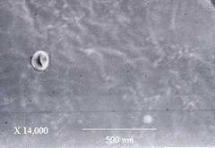
Table 1. Coded values of the formulation parameters of leuprolide acetate liposomes by 3x3 factorial design.
|
Coded values |
Actual values | ||
|
X1 |
X2 |
X3 | |
|
-1 |
0.25 |
0.05 |
0.13 |
|
0 |
0.5 |
0.2 |
0.2 |
|
1 |
1.0 |
0.5 |
0.5 |
|
Coded Values: -1, low level; 0, intermediate level; 1, high level. Actual values: X1 , Volume of aqueous phase (ml); X2 , HSPC: DSPG [Negative charge] (molar ratio); X3 ,HSPC: Cholesterol (molar ratio). | |||
Twenty seven batches of different combinations were prepared, by taking values of selective variables X1, X2 and X3 at different levels as shown in Table 1.The prepared batches were evaluated for percent drug entrapment (PDE), a dependent variable and the results are recorded in Table 2. Mathematical modeling was carried out by using equation 1 to obtain a second order polynomial equation (38).
Y= b0+b1X1+b2X2+b3X3+b12X11+b22X22+b32X33+b12X1X2+b13X1X3+b23X2X3+b123X1X2X3 (eq. 1)
where Y is the dependent variable (PDE) while b0 is the intercept, bi (b1, b2 and b3), bij (b12 , b13 and b23) and bijk (b123) represents the regression coefficient for the second order polynomial and Xi represents the levels of independent formulation variables. Prime independent formulation variables affecting the PDE in Reverse Phase Evaporation (REV) method were the volumes of aqueous phase (X1) and the ratios HSPC/DSPG (X2), and HSPC/Cholesterol (X3). Hence these variables were selected to find the optimized condition for higher PDE using 3x3 factorial design, and contour plots. A full model (equation 2) was established after putting the values of regression coefficients in equation 1.
Table 2: 3x3 full factorial design layout for the determination of percent drug entrapment in the formulation of liposomes.
|
Batch No. |
X1 |
X2 |
X3 |
X12 |
X22 |
X32 |
X1X3 |
X2X3 |
X1X2 |
X1X2X3 |
Y (PDE)* (+ S.E.M) |
|
1 |
-1 |
-1 |
-1 |
1 |
1 |
1 |
1 |
1 |
1 |
-1 |
48.94 (0.236) |
|
2 |
0 |
-1 |
-1 |
0 |
1 |
1 |
0 |
1 |
0 |
0 |
48.25 (0.352) |
|
3 |
1 |
-1 |
-1 |
1 |
1 |
1 |
-1 |
1 |
-1 |
1 |
46.80 (0.186) |
|
4 |
-1 |
0 |
-1 |
1 |
0 |
1 |
1 |
0 |
0 |
0 |
60.80 (0.050) |
|
5 |
0 |
0 |
-1 |
0 |
0 |
1 |
0 |
0 |
0 |
0 |
56.28 (0.036) |
|
6 |
1 |
0 |
-1 |
1 |
0 |
1 |
-1 |
0 |
0 |
0 |
50.43 (0.086) |
|
7 |
-1 |
1 |
-1 |
1 |
1 |
1 |
1 |
-1 |
-1 |
1 |
30.32 (0.074) |
|
8 |
0 |
1 |
-1 |
0 |
1 |
1 |
0 |
-1 |
0 |
0 |
24.67 (0.044) |
|
9 |
1 |
1 |
-1 |
1 |
1 |
1 |
-1 |
-1 |
1 |
-1 |
20.86 (0.102) |
|
10 |
-1 |
-1 |
0 |
1 |
1 |
0 |
0 |
0 |
1 |
0 |
42.25 (0.136) |
|
11 |
0 |
-1 |
0 |
0 |
1 |
0 |
0 |
0 |
0 |
0 |
42.56 (0.032) |
|
12 |
1 |
-1 |
0 |
1 |
1 |
0 |
0 |
0 |
-1 |
0 |
40.23 (0.122) |
|
13 |
-1 |
0 |
0 |
1 |
0 |
0 |
0 |
0 |
0 |
0 |
55.82 (0.075) |
|
14 |
0 |
0 |
0 |
0 |
0 |
0 |
0 |
0 |
0 |
0 |
50.32 (0.089) |
|
15 |
1 |
0 |
0 |
1 |
0 |
0 |
0 |
0 |
0 |
0 |
43.86 (0.032) |
|
16 |
-1 |
1 |
0 |
1 |
1 |
0 |
0 |
0 |
-1 |
0 |
26.83 (0.066) |
|
17 |
0 |
1 |
0 |
0 |
1 |
0 |
0 |
0 |
0 |
0 |
20.32 (0.056) |
|
18 |
1 |
1 |
0 |
1 |
1 |
0 |
0 |
0 |
1 |
0 |
19.23 (0.108) |
|
19 |
-1 |
-1 |
1 |
1 |
1 |
1 |
-1 |
-1 |
1 |
1 |
34.98 (0.205) |
|
20 |
0 |
-1 |
1 |
0 |
1 |
1 |
0 |
-1 |
0 |
0 |
38.86 (0.049) |
|
21 |
1 |
-1 |
1 |
1 |
1 |
1 |
1 |
-1 |
-1 |
-1 |
36.23 (0.036) |
|
22 |
-1 |
0 |
1 |
1 |
0 |
1 |
-1 |
0 |
0 |
0 |
50.23 (0.102) |
|
23 |
0 |
0 |
1 |
0 |
0 |
1 |
0 |
0 |
0 |
0 |
47.89 (0.112) |
|
24 |
1 |
0 |
1 |
1 |
0 |
1 |
1 |
0 |
0 |
0 |
43.56 (0.031) |
|
25 |
-1 |
1 |
1 |
1 |
1 |
1 |
-1 |
1 |
-1 |
-1 |
22.42 (0.098) |
|
26 |
0 |
1 |
1 |
0 |
1 |
1 |
0 |
1 |
0 |
0 |
17.68 (0.133) |
|
27 |
1 |
1 |
1 |
1 |
1 |
1 |
1 |
1 |
1 |
1 |
16.20 (0.056) |
|
*n=3. | |||||||||||
Model fitting and prediction
The PDE values were fitted to a second order polynomial model based on response surface regression. Response surface regression is a rapid technique used to empirically derive a functional relationship between an experimental response (PDE) and a set of input variables. Furthermore, it may determine the optimum level of experimental factors required for a given response. A factor is defined as an input variable whose value can be set during an experiment. The response variable is a measured quantity whose value is affected by levels chosen for the factors. Response surfaces that show the relationships between the response variable (PDE) and formulation variables were generated from the fitting.
Y=50.69–3.07X1–10.03X2–4.41X3–0.20X12–18.93X22+0.698X32+0.861X1X3+1.2X2X3–1.698X1X2-0.0188X1X2X3 (eq. 2)
The fitting results were statistically tested for lack of fit. Model simplification was carried out by eliminating non-significant parameters as shown in Table 3 (P<0.05) in the polynomial equations resulting from multiple regression analysis. Selection of the final model was based on three statistical parameters, the p-value of the test of lack of fit, the r2 value and the significance levels of individual parameters. The resulting reduced model was then used to predict the response variable (PDE) within the experimental range, especially at the experimental conditions where the maximum PDE was expected to be obtained.
Y=50.69–3.07X1-10.03X2-4.41X3–18.93X22–1.698X1X2+1.2X2X3 (eq. 3)
Results of ANOVA of full model and reduced model were carried out and the F-Statistic was applied to check whether the nonsignificant terms can be omitted or not from the full model which is shown in Table 4.
Contour Plots
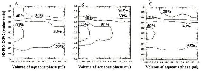
Two-dimensional contour plots were established using the polynomial equation (equation 2). Values of X1and X2 were computed at prefixed values of PDE. Three contour plots were established between X1and X2 at fixed level if -1, 0 and 1 level of X3 as shown in Figure 4 (A, B and C). The volume of the aqueous phase was plotted along the x-axis and the HSPC: DSPG molar ratio on the y axis and the corresponding percent drug entrapment (PDE) was plotted as line graph (contour plot).
Artificial Neural Network
A commercial Microsoft Window’s based ANN software package, Matlab 6.1 was used throughout the study with a Pentium 4 personal computer. Briefly, the general structure of the ANN has three input layers, one hidden layer and one input layer. Each layer has a few units corresponding to neurons. The units in the neighboring layers are fully interconnected with links corresponding to synapses. The strength of connections between two units are referred to as weights. In the hidden layer and output layer the processing unit sums its input from the previous layer and then applies the sigmoidal function to compute its output to the following layer according to the following equations
where wpq is the weight of the connection between unit q in the current layer to unit p in the previous layer, and xp is the output value of the previous layer. f(yq) is connected to the following layer as an output value. Alpha is a parameter relating to the shape of the sigmoidal function. Non linearity of the sigmoidal function is strengthened with an increase in α. ANN learns an approximate non-linear relationship by a procedure called training, which involves varying weight values. Training is defined as a search process for the optimized set of weight values, which can minimize the squared error between the simulation and experimental data of units in the output layer.
Model training, validation and optimization
A multi-layer feed forward back-propagation (39, 40) network that was created by generalizing the Levelberg-Marquardt’s learning rule to multiple layer networks and nonlinear differential transfer functions, was used to predict PDE of the liposomal formulations. The back-propagation (BP) learning algorithm is the most widely used training algorithm in multi-layered feed forward networks. A method called momentum decreases BP’s sensitivity to small details in the error surface. This helps the network avoid getting stuck in local minima, which would prevent the network from finding a lower error solution. The momentum helps the network to overcome obstacles (local minima) in the error surface and settles down at or near the global minima (solution with lowest possible error). Our network architecture consisted of an input layer with three neurons, an output layer with one neuron and a hidden layer (Figure 2).
Figure 2: The feed forward back-propagation network used in the study. X1, volume of aqueous phase, X2, HSPC: DSPG, X3, HSPC: Chol, Y, Percent drug entrapment (PDE); H1-H9, nodes of the hidden layer; W11, connection from first input node to the first hidden node; W11, connection from the first hidden node to the output node; W93, connection from the third input node to the ninth hidden node; W19, connection from the ninth hidden node to the output node.
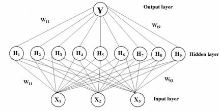
Figure 3: Squared correlation coefficients (r2) for 27 formulations as a function of the number of hidden nodes using ANN.
The network parameters (weights) are initially set to random values. During the training phase, the actual output of the network is compared with the desired output and the error propagated back toward the input of the network. A neural network has two phases, commonly referred to as the training phase and the prediction phase. During the training phase, sample data containing both inputs and the desired outputs are processed to optimize the network’s output meaning to minimize the deviation. The number of hidden nodes in a network is critical to network performance. Too few nodes can lead to under fitting. Too many nodes can lead the system towards memorizing the patterns in the data (41). According to Kolmogorov’s theorem, it is understood that twice the number of input nodes plus one is sufficient to compute any arbitrary continuous function. Input vectors and the output vector (response) were used to train the network until it can approximate a function, associate input vectors with specific output vectors. Initially one hidden layer was used and the number of hidden layer nodes was varied from 1-11, using 100 iterations. In order to select the optimum ANN model, regression plots were constructed for the observed vs. predicted PDE for the 27 test formulations. The ANN model that yielded a regression plot with a slope and r2 that were both closest to one was selected as the optimum ANN model.
In order to validate the ANN model, the model was trained again using 26 formulations and withholding one formulation. Once the ANN model was trained, the model predicted the PDE for the withheld formulation. This process was repeated 27 times, each time withholding a different test formulation from the training set. This validation method is called the “leave-one out method”. A regression plot was then constructed for the predicted PDE and observed PDE to obtain a slope and r2 to 1 as shown in Figure 3. The determination of the final optimized model was based on the slope and r2 values for all 27 formulations.
Normalized Error Determination:
The quantitative relationship established by both the techniques (ANN and MLR) was confirmed by preparing experimentally six liposomal formulations by random selection of causal factors. PDE predicted from the ANNs and MLR was compared with those generated from physical experiment using Normalized Error (NE). The equation of NE is expressed as follows:
NE = [S{(Pr - Er)/Er}2]1/2
where Pr and Er represents predicted and experimental response respectively.
RESULTS
By using 3x3 factorial design, twenty seven batches of leuprolide acetate liposomes were prepared by REV method by varying three independent variables, volume of aqueous phase (X1), HSPC: DSPG [molar ratio (X2)] and HSPC: Chol [molar ratio (X3)]. The percent drug entrapment (PDE), which was taken as dependent variable was determined and the results are recorded (Table 2). A substantially better drug entrapment achieved in liposomes prepared by REV method was 60.8% at -1 level of X1 (0.25ml), 0 level of X2 (1: 0.2) and -1 level of X3 (1:0.13) with the average particle size of about 180nm.The Scanning Electron Microscopy (SEM) shows that the particles are spherical in shape as shown in Figure 1.
Multiple linear regression:
The main effects of X1, X2 and X3 represent the average result of changing one variable at a time from its low to high value. The interactions (X1X2, X1X3, X2 X3 and X1 X2 X3) show how the PDE changes when two or more variables were simultaneously changed. The PDE values for the twenty-seven batches showed a wide variation from 16.2 to 60.8 % (Table 2). This is reflected by the wide range of coefficients of the terms of equation 2 representing the individual and combined variables. Small values of the coefficients of the terms X12, X32, X1X3, X1X2X3 in equation 2 were regarded as least contributing variables in the preparation of leuprolide acetate liposomes by REV technique. Hence, these terms were neglected from the full model considering non-significance and a reduced polynomial equation (equation 3) obtained following multiple regression of PDE and significant terms (p<0.05) of equation 2.
The significance of each coefficient of the equation 2 was determined by student ‘t’ test and p-value, which are listed in Table 3. The larger the magnitude of the t value and the smaller the p value, the more significant is the corresponding coefficient. This implies that the quadratic main effects of volume of aqueous phase (X1), HSPC: DSPG (X2) and HSPC: Chol (X3) are found to be very significant. The second order main effects of HSPC: DSPG are significant, as is evident from their p-values. The interaction between X2X3 and X1 X2 are found to be significant from their p-values (Table 3).
Table 3: Model coefficients estimated by multiple linear regression.
|
Factor |
Coefficients |
Computed t- value |
P-value |
|
Intercept |
50.69185 |
55.17267 |
1.10E-19* |
|
X1 |
-3.06611 |
-7.20904 |
2.08E-06* |
|
X2 |
-10.0317 |
-23.5864 |
7.42E-14* |
|
X3 |
-4.40556 |
-10.3583 |
1.68E-08* |
|
X12 |
-0.20389 |
-0.27677 |
0.785499 |
|
X22 |
-18.9306 |
-25.6976 |
1.95E-14* |
|
X32 |
0.697778 |
0.947209 |
0.35762 |
|
X1X3 |
0.860833 |
1.652581 |
0.117901 |
|
X2X3 |
1.1975 |
2.298895 |
0.035322* |
|
X1X2 |
-1.6975 |
-3.25877 |
0.004929* |
|
X1X2 X3 |
-0.01875 |
-0.02939 |
0.976917 |
|
* Significant at p < 0.05 | |||
Table 4: Analysis of variance (ANOVA) of full and reduced models of multiple linear regression.
|
DF |
SS |
MS |
F |
R |
R2 |
Adj R2 | ||
|
Regression |
FM |
10 |
4544.045 |
454.4045 |
139.56 |
0.994 |
0.989 |
0.982 |
|
RM |
6 |
4531.979 |
755.3298 |
235.44 |
0.993 |
0.986 |
0.982 | |
|
Error |
FM |
16 |
52.097(E1) |
3.256 |
139.56 |
|||
|
RM |
20 |
64.163(E2) |
3.208 |
235.44 | ||||
|
SSE2 – SSE1 = 64.163-52.097 = 12.066 No: of parameters omitted = 4 MS of Error (full model) = 3.256 F calculated = (12.066/4)/3.256 = 0.926 | ||||||||
The results of ANOVA of the second order polynomial equation are given in Table 4. F-Statistics of the results of ANOVA of full and reduced model confirmed omission of non-significant terms of equation 6. Since the calculated F value (0.926) is less than the tabulated F value (3.256) (a = 0.05, V1=4 and V2 = 16), it was concluded that the neglected terms do not significantly contribute in the prediction of PDE.
When the coefficients of the three independent variables in equation 2 were compared, the value for the variable X2 (b2 = -10.0317) was found to be maximum and hence the variable X2 was considered to be a major contributing variable for PDE of leuprolide acetate liposomes. The
Fisher F test with a very low probability value demonstrates a very high significance for the regression model. The goodness of fit of the model was checked by the determination coefficient (R2). In this case, the values of the determination coefficients (R2 = 0.989 for full model and 0.986 for reduced model) indicated that over 90 % of the total variations are explained by the model. The values of adjusted determination coefficients (adj R 2 = 0.982 for full model and 0.982 for reduced model) are also very high which indicates a high significance of the model. A higher values of correlation coefficients (R = 0.994 for full model and 0.993 for reduced model) signifies an excellent correlation between the independent variables.
Figure 4: Contour plots (A) at -1 level of variable X3, (B) at 0 level of variable X3, (C) at 1 level of variable X3.
 |
7Table 5: Test data set for validating ANN and MLR model for the determination of percent drug entrapment in the formulation of liposomes.
|
Formulation |
Vol. of Aqueous phase (X1)(ml) |
HSPC: DSPG (X2) |
HSPC: Cholesterol (X3) |
Experimental PDE (S.E.M) |
Predicted PDE (ANN-bp) |
Predicted PDE (MLR-from contours) |
|
1 |
1 |
1:0.26 |
1:0.13 |
48.23 (0.256) |
48.739 |
50.42 |
|
2 |
0.25 |
1:0.14 |
1:0.2 |
53.96 (0.196) |
54.606 |
54.7 |
|
3 |
0.45 |
1:0.14 |
1:0.5 |
47.36 (0.203) |
47.94 |
46.85 |
|
4 |
0.8 |
1:0.05 |
1:0.2 |
40.01 (0.189) |
39.898 |
40.44 |
|
5 |
0.3 |
1:0.17 |
1:0.5 |
48.73 (0.162) |
48.889 |
50.19 |
|
6 |
0.35 |
1:0.08 |
1:0.13 |
50.23 (0.208) |
49.637 |
49.07 |
|
“t” calculated |
0.3611 |
0.3451 | ||||
|
“t” tabulated |
2.5706 | |||||
|
Normalised error |
0.0211 |
0.0658 | ||||
|
*n=3 |
||||||
Contour plots
Figure 4A shows the contour plot drawn at -1 level of X3 (1:0.13) for a prefixed PDE value of 30%, 40%, 50%, and 60%. The plots were found to be linear for 30 %, 40% and 50% but for 60 % PDE the plots were found to be non-linear having upward and downward segment signify non-linear relationship between volume of aqueous phase (X1) vs. HSPC/DSPG (X2) variables. It was determined from the contour that maximum PDE (60%) could be obtained with X1 range at – 1 level to – 0.6 level (0.25ml to 0.35ml) and with X2 range at - 0.2 level to 0.2 level (1:0.17 to 1: 0.26) when X3 (1:0.13) was used.
Figure 4B shows the contour plot drawn at 0 level of X3 (1:0.2) for a prefixed PDE value of 20%, 30%, 40%, 50% and 55%. The plots were found to be linear for 20 %, 30% and 40% but for 50 % and 55% PDE the plots were found to be non-linear having upward and downward segment signify non-linear relationship between X1 and X2 variables. It was determined from the contour that maximum PDE (55%) could be obtained with X1 range at – 1 level to – 0.6 level and with X2 range at – 0.2 level to 0.2 level.
Figure 4 C depicts the contour plot drawn at 1 level of X3 (1:0.5) for a prefixed PDE value of 20%, 30%, 40%, and 50%. The plots were found to be linear for 20 %, 30% and 40% but for 50 % PDE the plots were found to be non-linear having upward and downward segment signify non-linear relationship between X1 and X2 variables. It was determined from the contour that maximum PDE (50%) could be obtained with X1 range at – 1 level to – 0.6 level and with X2 range at – 0.2 level to 0.2 level.
ANN structure
A multi-layer feed forward back-propagation network using Levelberg-Marquardt’s learning rule was used to predict PDE of the liposomal formulations. Three causal factors corresponding to different levels of the volume of aqueous phase (X1), HSPC/DSPG [negative charge] (X2), and HSPC/Cholesterol (X3) were used as each unit of the input layer in the ANN. PDE were used as output layer. The output layer was composed of one response variable, Y, percent drug entrapment (PDE). A set of PDE and causal factors was used as tutorial data for ANN and fed into a computer. Several training sessions were conducted with different numbers of nodes of hidden layer and training times in order to determine the optimal ANN structure (42,43). For selecting the number of hidden nodes, we started of with 1 hidden node and we gradually increased the number of nodes until a network of least mean squared error was attained. Increase in number of nodes led to decrease in least mean squared error. The learning period was completed when minimum root mean square (RMS) was reached.
RMS = [∑ (yip - yim)2 /n]1/2 (eq. 6)
Where yip is experimental (observed) response, yim is calculated (predicted) response, and n is number of experiments. The RMS reached after the training was 0.0000354, which is found to be minimum. Further increase in hidden nodes produced high error, when the network was validated with another set of test data (Table 5). Figure 3 shows a representative plot of r2 values for an ANN model prediction performance as a function of number of nodes in the hidden layers. In this case, an ANN with 9 nodes in the hidden layer resulted in slope and r2 values that are closest to 1.0.The student ‘t’ test carried out between the predicted results (t value = 0.3611) from the ANN and the experimental results showed no statistically significant difference between them. The normalized error (NE) between the predicted and experimental response variables was employed as an evaluation standard between ANN and MLR. The NE value observed with the optimal ANN structure was 0.0211, while it was 0.0658 in case of second order polynomial equation (MLR).
Comparison of ANN and MLR:
Both ANN and MLR visualized similar results and their predictions regarding the PDE coincided very well. To check the accuracy of these predictions, we prepared experimentally six liposomal formulations by random selection of causal factors. Experimental results were comparable to the predicted results (Table 5).
Data analysed using paired students ‘t’ test revealed that there was no statistically significant difference between the experimental results and the predicted results of ANN (t = 0.3611) and MLR (t = 0.3451).
DISCUSSION
Multiple linear regression
The PDE (dependent variable) obtained at various levels of three independent variables (X1, X2 and X3) were subjected to multiple regression to yield a second order polynomial equation (full model). Multiple linear regression indicated a strong correlation between the PDE and each of the experimental variables. It also indicated strong interactions between these variables, which are represented by the interaction terms in the fitting equation (equation 2).
ANN
ANN is biologically inspired, that is, researchers are usually thinking about the organization of the brain when considering network configurations and algorithms. The human brain consists of neurons (@ 1011), which are interconnected in very complex manner (@ 1014 connections per neuron). Artificially implementing this structure to mimic human behaviour is ANN. An ANN consists of one or more layers of simple processing elements called neurons, neurodes or simple nodes. A node has an output and several inputs. Each input is multiplied by its weight and summed together and called as Network output or NET. The NET is passed through a transfer function is the sigmoid function defined as follows.
F (NET) = 1/(1+e-NET)
Depending upon the architecture in which individual neurons are connected; there are several types of ANNs. The most widely use architecture is multiplayer Back Propagation ANN (BPA) (44-47). It consists of an input layer, an output layer and one or more layers in between the input and output layers, called hidden layers. To train an ANN, initially all the weights are assigned random values and the input and the desired output vectors are presented to the ANN. ANN uses the input vector to produce an output vector. The output vector is compared with the desired output to calculate the error vector E. Training is accomplished by sequentially applying input vectors, while adjusting network weights according to a predetermined procedure. During training, the network weights gradually converge to values such that each input vector produces the desired output vector. Training of the network is called learning. There are two types of learning for the ANN viz. supervised learning and unsupervised learning. BPA is used to train the multiplayer ANN and uses supervised learning. Our network architecture consisted of an input layer with three neurons, an output layer with one neuron and a hidden layer of 9 neurons. Figure 2 shows the three layer ANN, where X1, X2, and X3 are inputs to the network, H1 to H9 are the 1st to 9th hidden layer and Y output layer of the network respectively; W1, W2, W3, W19 are the weights; The weight changes DWij for each input pattern Ij is given by
DWij = g(zI – Oi) Ij
(zi – Oi) = di = errors
Where zi is the target value and Oi is the output value of the elements and g is the learning rate. The derivatives of the errors, called d values, are calculated for the network’s output layers, and then back propagated through the network until d vectors are approximated for the hidden layers. Hence this learning rule is popularly known as d back propagation rule (48). Trained back-propagation networks tend to give reasonable answers when presented with inputs that they have never seen. We chose sigmoidal transfer function in our network, because it is nonlinear in nature and is well suited as a back propagation transfer function. The set of weight values was identified by gradient descent method. This method involves a continual change of values of the weights and biases in the direction of the steepest error descent called global error minimum.
Comparison of ANN and MLR:
A close look of both ANN and MLR reveals following facts. An ANN can be used for linear and nonlinear systems. Its use allows us to study the covariate interactions. By adjusting weights, multivariate outputs can also be evaluated. It uses slopes and intercepts to ascertain the variable response relationship. The normalized error obtained from ANN was less, compared to the multiple regression analysis shows the higher accuracy in prediction. ANN can easily handle more input variables and extremely helpful when the numbers of experiments are more, but in case of MLR a large number of input variables lead to a polynomial with many coefficients that involves tedious computation. Another major advantage with ANN is the flexibility to work with the theoretical data for better prediction, but MLR does not accommodate theoretical or historical data.
This study demonstrated that MLR using second order polynomial equation and feed forward back-propagation network (ANN) are useful tools to understand the effects of the various formulation parameters in the preparation of leuprolide acetate liposomes by reverse phase evaporation method and to predict the best composition for a particular response. A three-layered 3-9-1 feed forward neural network was found to be an adequate descriptor of the PDE. The program was trained until the RMS was minimum and r2 was closest to 1.0. One method is complimentary to the other, with each having its own advantages. The established relationship was confirmed by preparing another set of six liposomal formulations having predetermined PDE. When experimental data were compared with predicted data by paired “t” test, no statistically significant difference was observed. ANN was found to be better in the prediction of PDE because the values of Normalised Error (NE) are lower for ANN modes compared to the MLR. In data analysis neural network appeared to be less biased and more precise, compared with MLR. This demonstrated the role of ANN & MLR in prediction of optimum formula of leuprolide acetate liposome formulation with predetermined PDE.
ACKNOWLEDGEMENTS: This research work was funded by the
University Grants Commission,
REFERENCES:
1. Levison, K.K., Takayama, K., Isowa, K., Okabe, K., Nagai, K. Formulation optimization of indomethacin gels containing a combination of three kinds of cyclic monoterpenes as percutaneous penetration enhancers. J. Pharm. Sci. 83: 1367-1372, 1994.
2.
Shirakura,
O., Yamada, M., Hashimoto, M., Ishimaru, S., Takayama, K., Nagai, K. Particle
size design using computer optimization technique. Drug.
3. Takahara , J., Takayama, K., Isowa, K. and Nagai, T., Multi-objective simultaneous optimization based on artificial neural network in a ketoprofen hydrogel formula containing O-ethylmenthol as a percutaneous absorption enhancer. Int J. Pharm., 158: 203-210, 1997.
4. Takahara, J., Takayama, K. and Nagai, T., Multi-objective simultaneous optimization technique based on an artificial neural network in sustained release formulations. J Contr Rel., 49: 11-20, 1997.
5.
Achanta,
A.S., Kowalski, I.G. and
6. Gobburu, J.V.S. and Shelver, W.H., Quantitative structure pharmacokinetic relations(QSPR) of beta blockers derived using neural networks. J. Pharm. Sci., 84(7): 862-865, 1995.
7. Veng-Pederson, P. and Modi, N. B., Application of neural networks to pharmacodynamics. J. Pharm. Sci., 82 (9): 918-926, 1993.
8. Gobburu, J.V.S. and Chen, E.P., Artificial neural networks as a novel approach to integrated pharmacokinetic-pharmacodynamic analysis. J. Pharm. Sci., 85 (5): 505-510, 1996.
9. Takayama, K., Morva, A., Fujikawa, M., Hattori, Y., Obata ,Y. and Nagai, T., Formula optimization of theophylline controlled-release tablet based on artificial neural networks. J Contr. Rel., 68: 175-186, 2000.
10. Chien, Y., McCall, T.W., Baichwal, A.R. and Meyer, M.C., The application of an artificial neural network and pharmacokinetic simulations in the design of controlled release dosage forms. J Contr. Rel., 68: 175-186, 2000.
11. Khawla, A., Abu,
12. Khuri, A.I. and Cornell,
J.A., Response Surfaces: Designs and Analysis. Marcel Dekker:
13. Chrisp, P. and Sorkin, E.M., Leuprorelin. A review of its pharmacology and therapeutic use in prostatic disorders. Drugs Aging., 1(6): 487-509,1991.
14. Oesterling, J.E., LHRH agonists. A nonsurgical treatment for benign prostatic hyperplasia. J Androl., 12(6): 381-388, 1991.
15. Tunn, U.W., Bargelloni, U., Cosciani, S., Fiacavento, G., Guazzieris, and Pagano, F., Comparison of LHRH analogue 1 month depot and 3-month depot by their hormonal levels and pharmacokinetic profile in patients with advance prostate cancer. Urol Int., 60(Suppl. 1): 9-16, 1998.
16. Garnick, M.B., Leuprolide versus diethyl stilbestrol for metestatic cancer. N. Engl J Med., 311: 1281-1286, 1984.
17. Okada, H., Sakura, Y., Kawaji, T., Yashiki, T. and Mima, H., Regression of rat mammary tumors by a potent leutinizing hormone releasing hormone administered vaginally. Cancer Res., 43: 1869-1874, 1983.
18. Redding, T.W. and Schally, A.V., Inhibition of prostate tumor growth in two rat models by chronic administration of D-Trp6 analogue of LHRH. Proc Natl Acad Sci. USA., 78: 6509-6512, 1981.
19. Langer, R. Bioavailability of
macromolecular drugs and its control. In: V.R. Smolen (Ed.), Controlled Drug
Bioavailability. Vol 3, John Wiley and Sons,
20.
21. Meyer, J., Whitcomb, L. and Collins, D., Efficient encapsulation of proteins within liposomes for slow release in vivo. Biochem. Biophys. Res. Commun., 199: 433-438, 1994.
22. Murramatsu, K., Maitani, Y.,
Takayama, K. and Nagai, T., The relationship between the rigidity of the
liposomal membrane and the absorption of insulin after nasal administration of
liposomes modified with an enhancer containing insulin in rabbits. Drug
23. Kato, Y., Hososkawa, T., Hayakawa, E. and Ito, K., Influence of liposomes on tryptic digestion of insulin. Biol. Pharm. Bull., 16: 457-461, 1993.
24. Papahadjopoulos, D. and Gabizon,
A.A., Sterically stabilized (Stealth®) liposomes: Pharmacological properties and
drug carrying potential in cancer, in liposomes as tools in basic research and
industry. Philippot, J.R., Schuber, F., (eds), CRC Press:
25. Martin, F.J., Clinical
pharmacology and antitumor efficacy of DOXIL (pegylated liposomal doxorubicin),
in Medical Applications of Liposomes. Lasic, D.D. and Papahadjopoulos, D.,
(eds),
26.
27. Mayer, L.D., Cullis, P.R. and Bally, M.B., The use of transmembrane pH gradient-driven drug encapsulation in the pharmacodynamic evaluation of liposomal doxorubicin. J. Liposome Res., 4: 529-553, 1994.
28. Abra, R.M. and
29. Allen, T.M., Mehra, T., Hansen, C. and Chin, Y.C., Stealth Liposomes: an improved sustained release system for 1--D-arabinofuranosylcytosine. Cancer Res., 52: 2431, 1992.
30. Zou, Y., Ling, Y.H., Van, N.T., Priebe, W. and Perz, S.R., Anti tumor activity of free and liposome entrapped annamycin, a lipophilic antracycline antibiotic with non cross resistance properties. Cancer Res., 54: 1479 – 1484, 1994.
31. Subramanian N, Archit Y and Murthy R.S.R., Artificial neural network as an alternative to multiple regression analysis in optimizing formulation parameters of cytarabine liposomes. AAPS PharmSciTech 5(1) article 4, 1-9, 2004.
32. Matthews, R.J., Scott, R.G. and Morgan, S.L., Characterization of an enzymatic determination of arsenic (V) based on response surface methodology. Anal.Chim.Acta., 133: 169-182, 1981.
33. Fannin, T.E., Marcus,
M.D.,
34. Szoka, F. and Papahadjopoulos,
D., Procedure for preparation of liposomes with large internal aqueous space and
high capture by reverse phase. Proc Natl Acad Sci..,
35. Adjei, A.L. and Hsu, L.,
Leuprolide and other LHRH analogues. Stability and characterization of protein
and peptide drugs: John, Y.W., Pearlman, R., eds. Plenum Press:
36. New, R.R.C., Liposomes a
practical approach IN: preparation of liposomes edited by New, R.R.C.,
37. Bligh, E.G., Dyer, W.J. A rapid
method of total lipid extraction and purification.
38. Anthony, A.N. and James, K.C.,
Pharmaceutical experimental design and Interpretation. Taylor and Francis
Publishers:
39. Rumelhart, D. E., Hinton, G. E., Williams, R. J. Learning internal representations by error propagation, Parallel distributed processing: explorations in the microstructure of cognition, vol. 1: Foundations, MIT Press, Cambridge, MA, 1986.
40. Werbos, P. J. Generalisation of Back Propagation with Application to a Recurrent Gas Market Model, Neural Networks, 1, 339-356, October 1988.
41. Erb, R.J. Introduction to backpropagation neural network computation, Pharm. Res., 10: 165–170, 1993.
42. Jha, B.K., Thambe. S.S. and Kulkarni, B.D., Estimating diffusion coefficients of a micellar system using an artificial neural network. J.Colloid Interfac. Sci., 170: 392-398, 1995.
43. Pradeep.S., Jurgen, V. Comparison of neural network and multiple linear regression as dissolution predictors. Drug Develop Indust Pharm., 29(3): 349-355, 2003.
44. Khiang, P.K., Penng, L.C., San, Q.S., Hock, K.K., Use of artificial network to predict drug dissolution profiles and evaluation of network performance using similarity factor. Pharm. Research., 17: 1384-1388, 2000.
45. Yixin, C., Tianjie, J., Troy, W.M., Anand, R,B., Marwin, C, M. Comparison of four artificial neural network software programs used to predict the in vitro dissolution of controlled release tablets. Pharmaceutical Development Technology., 7(3), 373-379, 2002.
46. Tuncer, D., Jonatham, H., Sibel,
47. Sveltana, I., Milica, J., Zorica, D., Jelena, P., Slobodan, D.P., Ljiljana, S., Biljana, S. Artificial neural networks in the modeling and optimization of aspirin extended release tablets with eudragit L 100 as matrix substance. AAPS Pharmscitech. 4(1): 62-70, 2003.
48. Hertz, J., Krogh, A., Palmer,
R.G., in: Introduction to the Theory of Neural computation.
Addison-Wesley:
Corresponding author: Dr. R.S.R. Murthy, Pharmacy Department, Donor’s Plaza, Opp. to University Main Office, M.S. University of Baroda, Fatehgunj, Vadodara-390 002, India, e.mail: murthyrsr@sify.com
Published by the Canadian Society for Pharmaceutical Sciences.
Copyright © 1998 by the Canadian
Society for Pharmaceutical Sciences.
http://www.cspscanada.org/
CSPS Home | JPPS Home | Search | Subscribe to JPPS