Vizualization of Internal Solitary Waves using Light Refraction
|
Experiments and Research performed by Danilo Fabres Pezzin and Sahith Reddy,
May 2014 - August 2014,
Departments of Physics and of Earth & Atmospheric Sciences, University of Alberta
|
Experimental Set-up
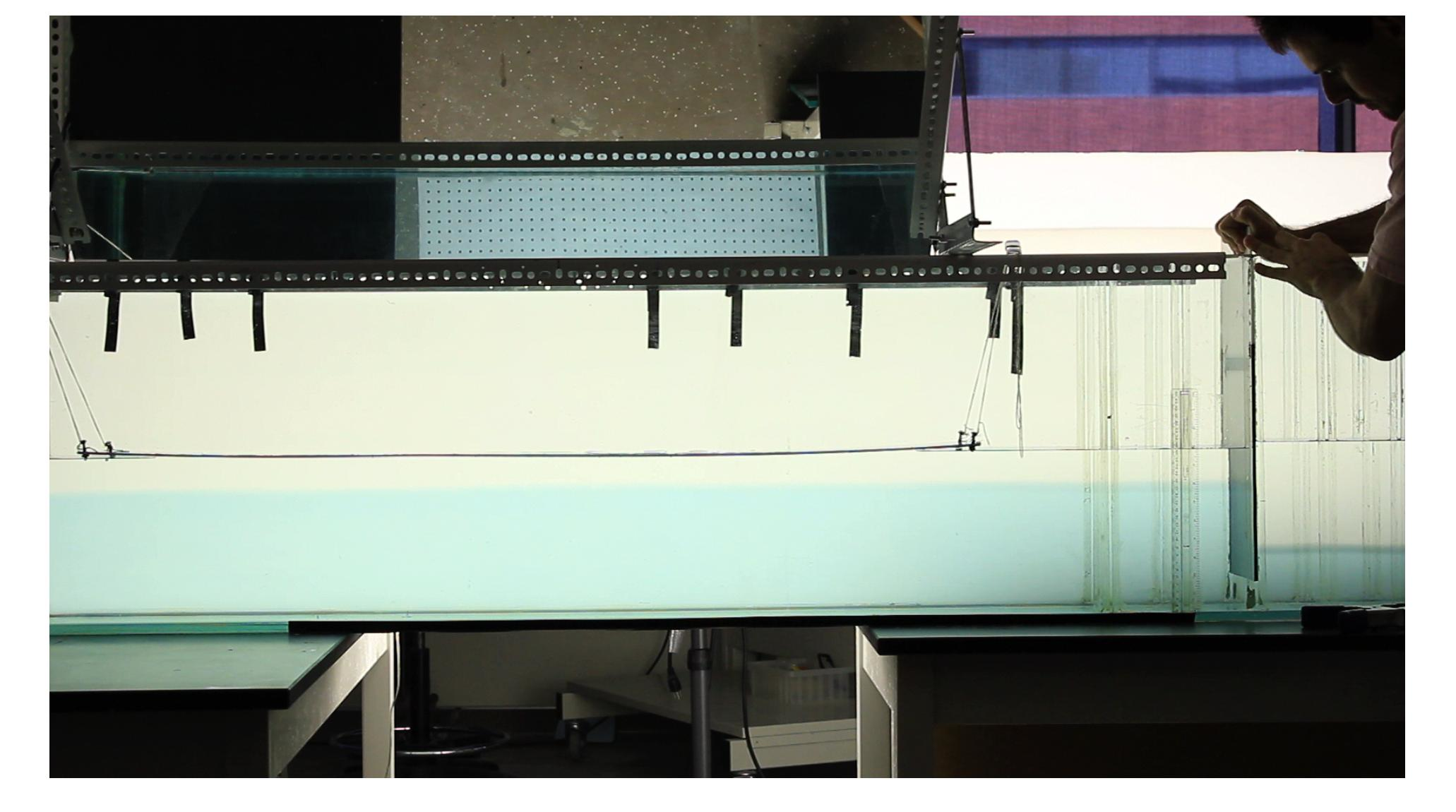
The experiment was performed in a tank with dimensions (L:W:H) of 197.0:17.5:49.0cm containing two different fluids. The upper fluid
is fresh water and the lower fluid is salt water. We filled the tank with approximate 15.0cm of fresh water and salt. After that it was
well mixed, we added approximate 5.0cm of fresh water and pulled the gate down (it was 28.5cm far from the right side of the tank and it
did not touch the tank's bottom). Then, we started to put more fresh water on the right side of the gate do create a different level
of the salt water between both side of the gate. In the next step, we laid a transparent acrilic sheet on the water surface to avoid
any kind of surface disturbance when the gate was pulled up. We placed a mirror with dimensions (L:H) of 122.0:62.0cm above the tank.
This mirror will reflect the dot sheets that were on the floor just beneath the tank, and the tank was 76.5cm from the floor. We placed
white sheet just behind the tank, so we were able to differ the interface between the two layers, and a light source behind this white
sheet (Figure 1).
Figure 1: Front and Top view of tank (the wave completely above the dot sheets).
(click on the image for experiment demonstration)
The main idea here is to catch the light that left the dot sheets, passed through the two fluid layers, was reflected by the mirror and
arrived at the camera's lens. Because of the wave, we will have distortion of the dots' position. Then, with the Matlab software, we
processed the frames of the movie in a way to recognize and to take the dots' position. The Figure 2.1 represents a snapshot
of the dots sheets at the initial moment and the Figure 2.2 a snapshot at t=7s.
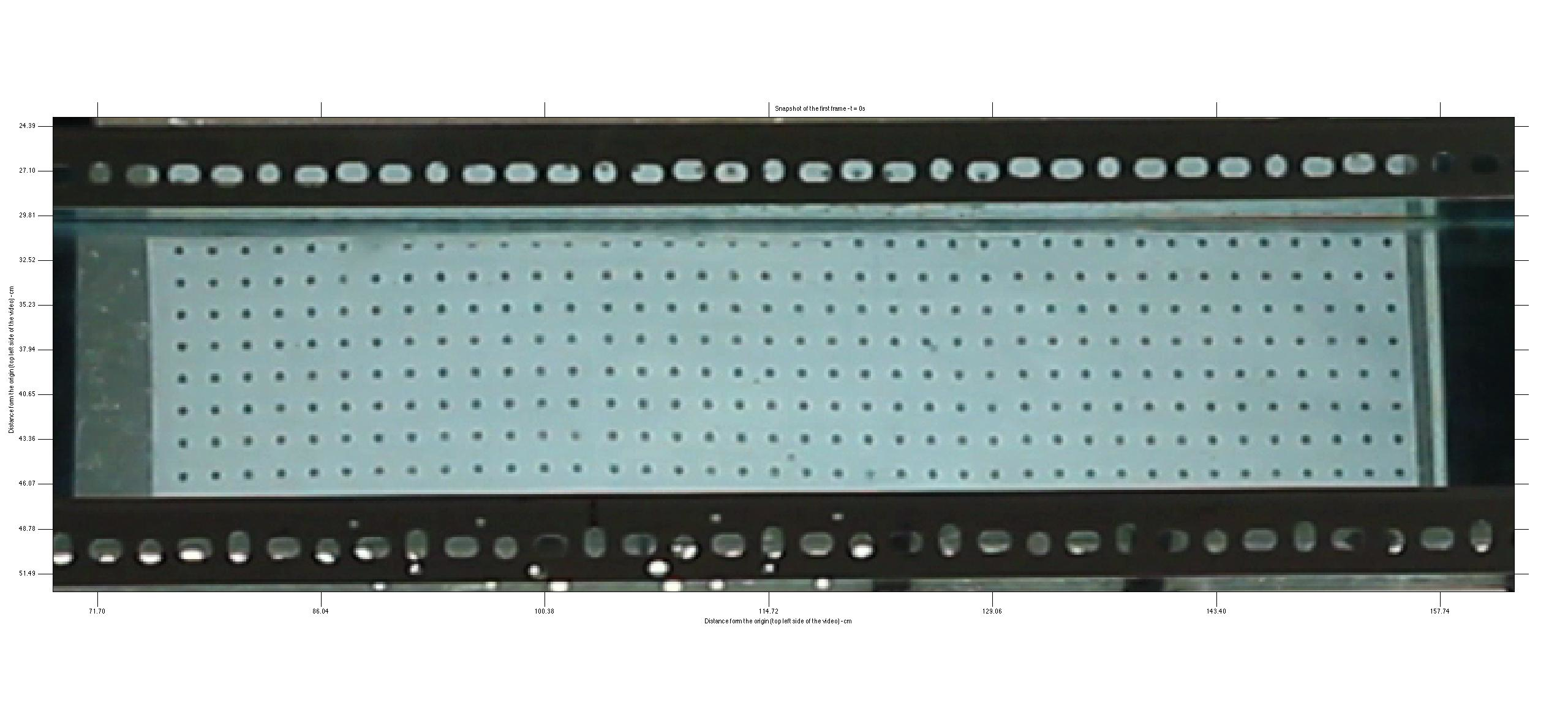
Figure 2.1: Snapshot of the dot sheets at t = 0s.
|
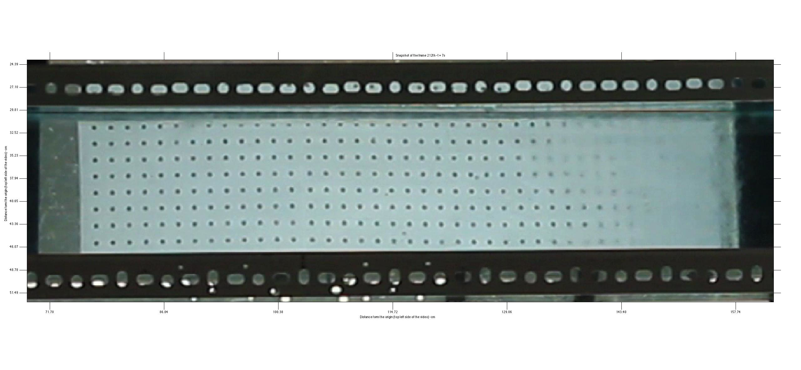
Figure 2.2: Snapshot of the dot sheets at t = 7s.
|
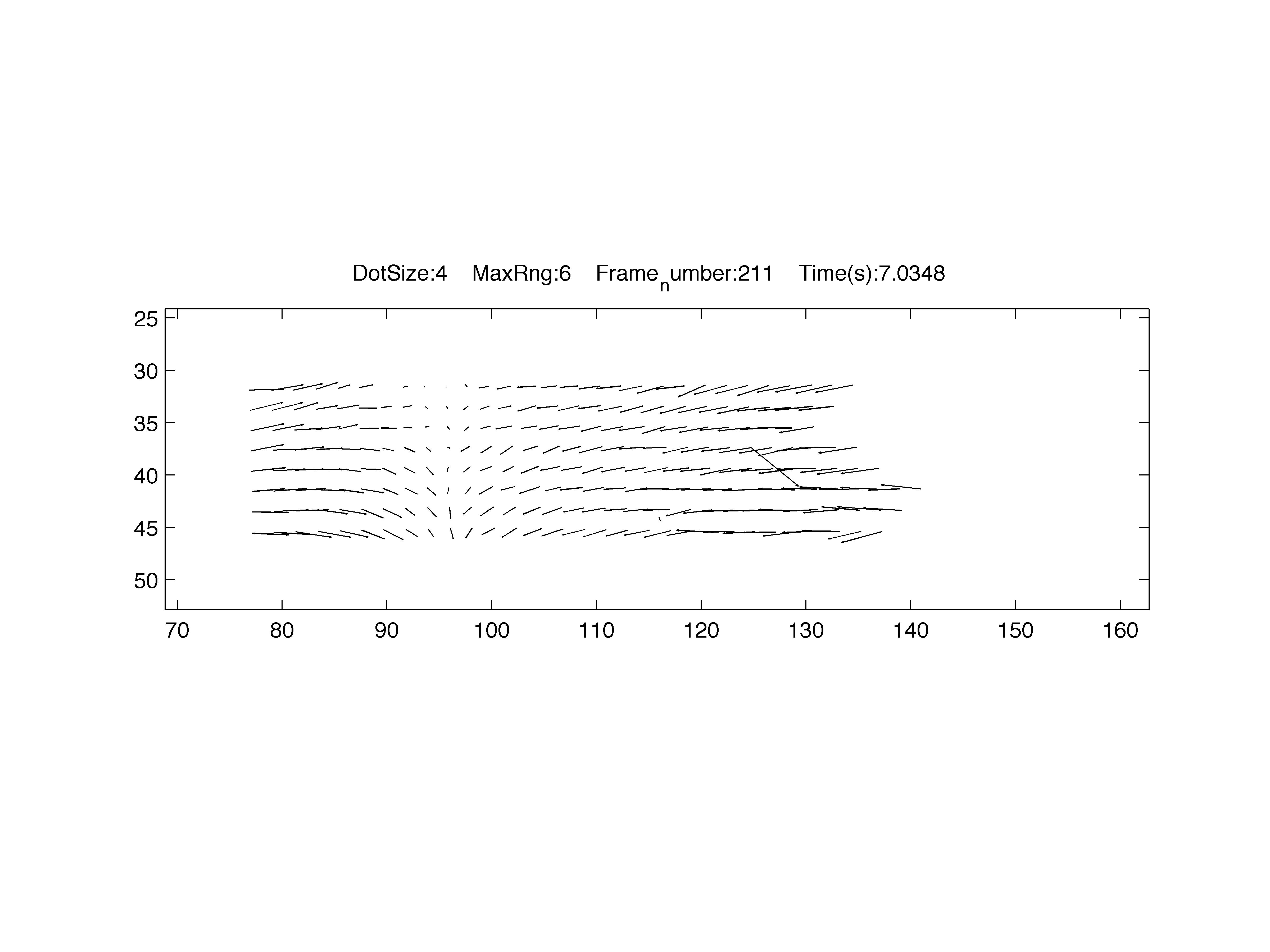
Figure 3: Displacement calculated between the dots' position at t = 0s and t = 7s.
|
The final part is to estimate the trough of the wave and make a theoretical calculation of the displacement. Then we will plot the
experimental and theoretical displacement to make sure that they match. The Figure 4.1 represents the image used to track the wave and
the Figure 4.2 represents the trough of the wave that was found. Now, it is needed to smooth the wave found because these big gradients
will not give right values of displacement when we start to calculate the theoretical displacement.
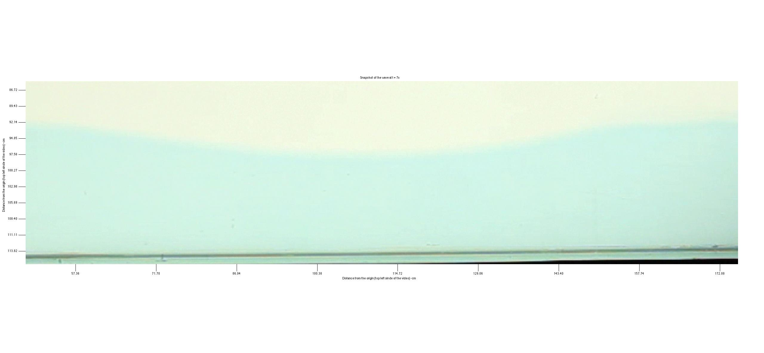
Figure 4.1: Snapshot of the wave at t = 7s.
|
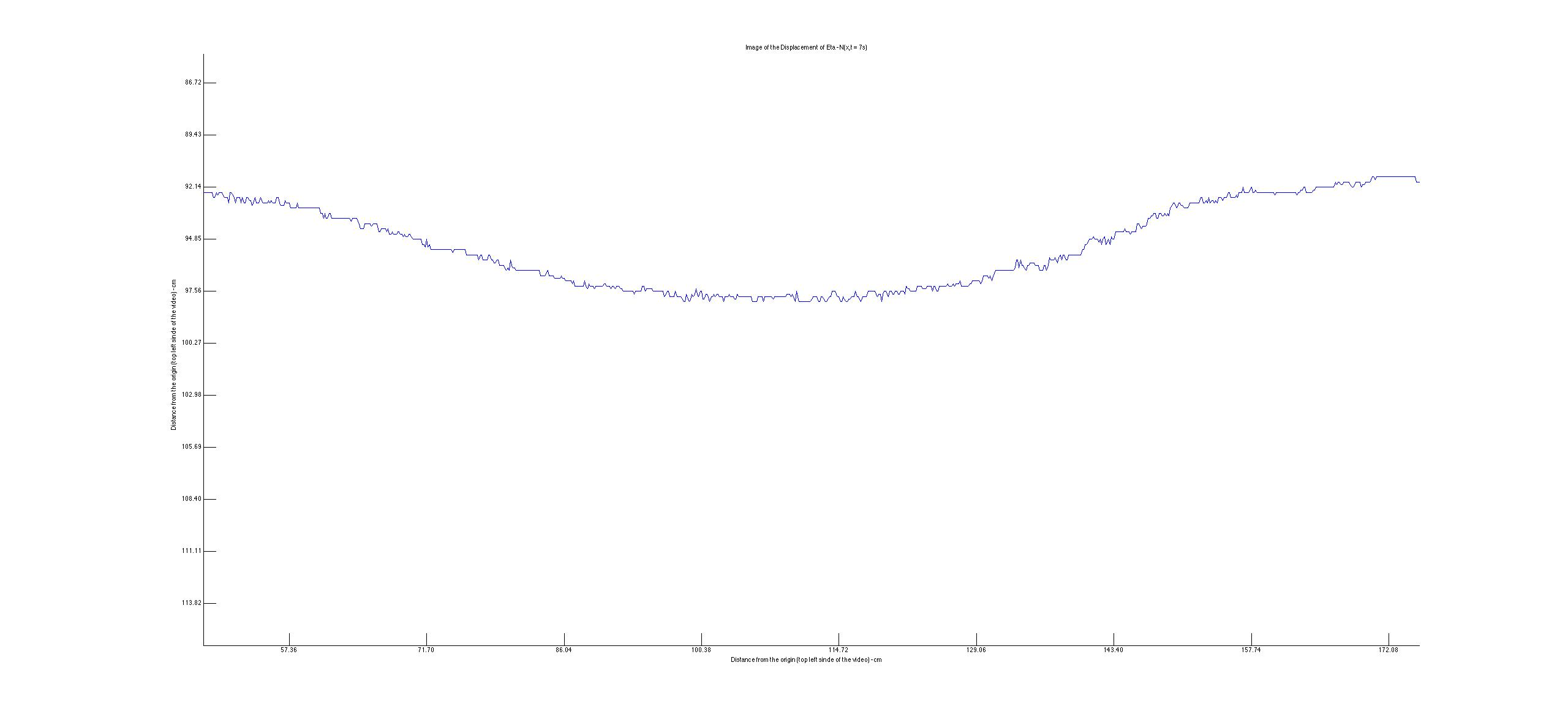
Figure 4.2: Image of the displacement of Eta - N(x,t = 7s).
|
Theory
The theory behind this experiment is the Snell's Law that is the following equation:
sin(θ1) n1 = sin(θ2) n2 . In other words, every
time that the light changed the environment the Snell's Law was applied. The Figure 5.1 and Figure 5.2 represent how it is processed the
theoretical calculation of the displacement. The Figure 5.3 represents where is placed all the equipament to drive the experiment.
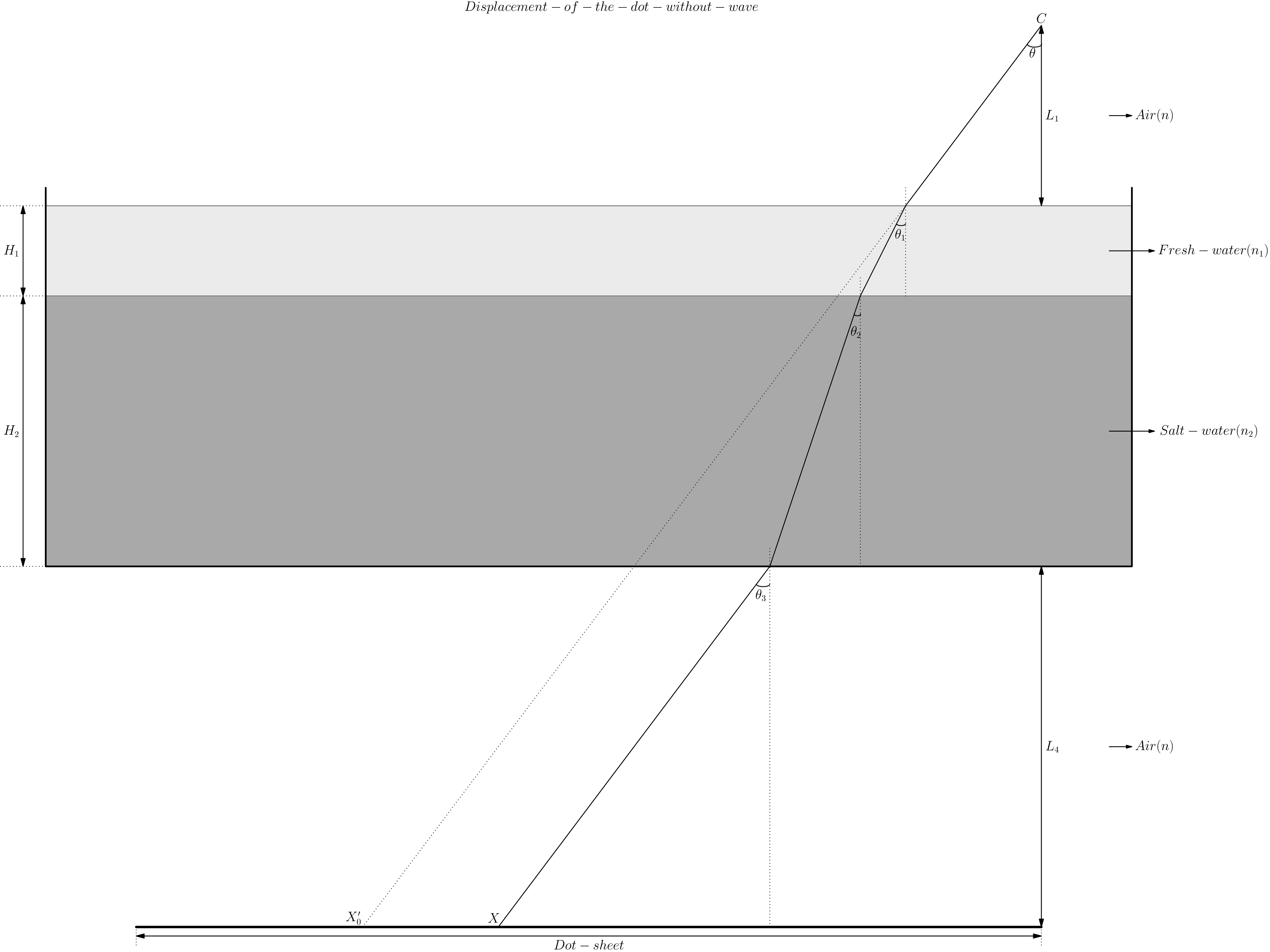
Figure 5.1: Dispacement of the dot without wave.
|
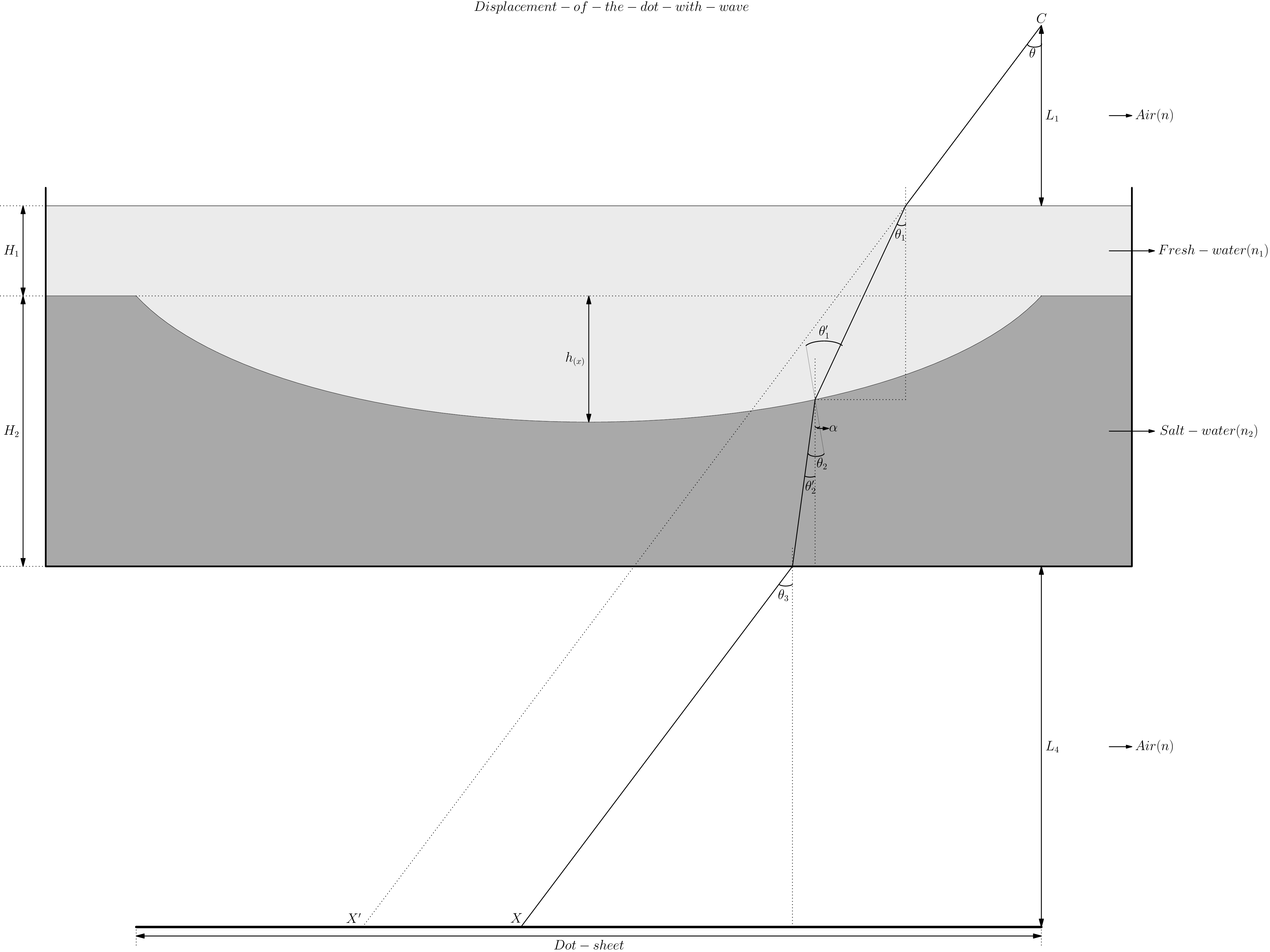
Figure 5.2: Displacement of the dot with wave.
|
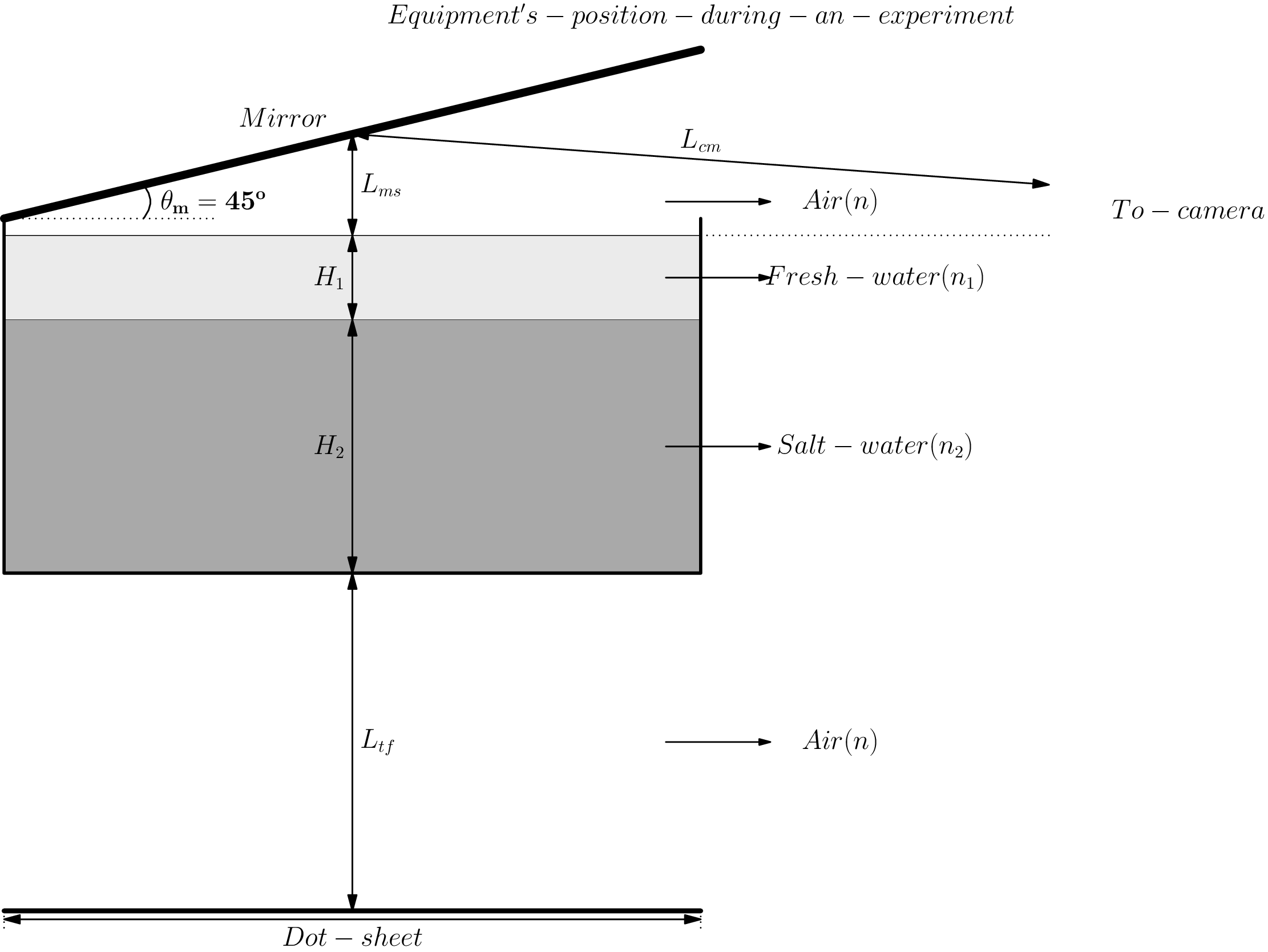
Figure 3: Equipment's position during an experiment.
|
Variabes explanation:
- H1 is the height of the upper layer.
- H2 is the height of the lower layer.
- h(x) is the trough of the wave for each position of x.
- Lcm is the distance between que camera (C) and the mirror.
- Lms is the distance between que the mirror and the water surface.
- Ltf is equal L4 and they are the distance between que the tank and the floor.
- L1 = Lcm + Lms
- X is the physical position of a dot.
- X0' is the position that the camera sees the dot without wave.
- X' is the position that the camera sees the dot with wave.
- The final displacement is give by: DISP = X' - X0'
- θ, θ1, θ2 and θ3 are the angles that the light arrives
at the camera as it goes through the different environment.
- θ1' = θ1 + α
- θ2' = θ2 - α
- α is the inclination of the wave at the position x and it is given by: α = ∂h(x) /
∂x
Results
Unfortunately, we could not finish the final part of the project.It consists to calculate the displacement with the theretical approach.
Hence, we did not do the comparation between the theoretical and experimental displacement.
Acknowledgements
This research was financially supported by the Brazilian Government through the government body CNPq (Conselho Nacinal de Desenvolvimento
Cientifico e Tecnologico).
I am very thankful for this opportunity given by Dr. Bruce Sutherland and for all the knowledge and experience that I learned during this 4
months working with him and his amazing research group.
Return to
Research Interests page
Bruce's home page
Department of Physics
Department of Earth and Atmospheric Sciences