EDIT202 – Spreadsheet Lab

Assignment Guidelines

---

Getting Started

1. For this lab you will modify a sample spreadsheet file named “Starter-SpreadSheet.xlsx” which is available for download from the Spreadsheet lab section on the Moodle site.

• Download this file to the computer (if you are working from lab on campus be sure to select Save As … from the File menu and save it to a safe location that will not be deleted upon re-start).

2. Using Microsoft Excel create a marking spreadsheet of a fictional class that meets the following guidelines. Name this file “LABSEC-CCID-SpreadSheet.xlsx”.

· Launch Microsoft Excel by opening the Starter-Spreadsheet.xlsx file. To open the file, locate it on your computer (wherever it was saved to in the previous step) and double click to open the file and launch Excel.

· Once you have launched Microsoft Excel you should see the program interface with a worksheet labeled “Starter-Spreadsheet.xlsx”.

· To save this file with a different file name select Save As... from the File menu.

Worksheet 1 – Student Marks

1. To calculate the percentages for each student you will need to insert a new column to the right of each “Raw Marks” column and label it “Percent”.

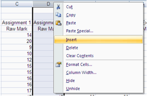
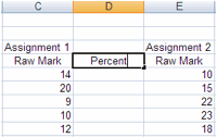
· To insert a new column, right click on a column header and select Insert from the available context menu.

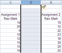
· The column will be inserted to the left. For example in the sample above the column would be inserted between column C and D.

· To enter information into a spreadsheet, click the mouse on the cell where you want data to appear, then type in Percent.

2. In the “Percent” columns, create a formula that will calculate the first student's percentage for that assignment or exam (Raw Mark / Marked Out Of). Use relative and absolute cell referencing.

· In order to properly use formulas all formulas must start with an equal sign, e.g. =B5-B20.

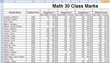
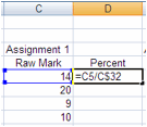
· When typing in formulas, the formula should be typed where you want the result to be displayed. For example in the sample sheet below to calculate the first percentage the correct formula would be, =C5/C$32 and the formula would be typed in under the Percent column.

· As an alternate to typing out each cell reference you can use your mouse. Once you begin a formula by entering an equal sign, then click your mouse on a cell you wish to use as a cell reference. You should notice that the cell reference is automatically entered into the formula. (This means when you are done your formula hit enter on the keyboard instead of clicking on another cell.)

· A relative cell reference is automatically adjusted when copying a formula to other cells. For example, if the following formula, = A1+B1 was copied, from cell C1 down to C2, the formula when copied would change to = A2+B2

· An absolute cell reference refers to a value that does not change when being copied to other cells. For example, if the following formula, =A$1+B$1 was copied, from cell C1 down to C2, the formula when copied would still be = A$1+B$1. In Microsoft Excel absolutes are represented as dollar signs, $).

· The absolute value in the percentage equation is the Marked Out Of value in cell C32. This is the value that each of the students’ Raw Scores will be divided by.

· Using this information it will be up to you to think of where to place the absolute ($).

3. Copy the formula down the column so that it determines the percentage for each student.

· To copy a formula, click on the bottom right-hand corner of the cell that needs to be copied and a little black crosshairs will appear.

· Drag down to include all the cells in the range.

· Release the mouse and we see our formula successfully copies with the correct results in our chosen cells.

4. Format each students’ percentage to be displayed in percent format and to include one decimal place (e.g. 65.4% not 0.654).

· To get all of the numbers on your spreadsheet displayed in a consistent manner, such as an equal number of decimal places, you need to set a number formatting option.

· To do this, first highlight the whole block of cells you want to format. The cells do not need data in them to complete this step; any data entered later will be formatted in this manner.

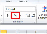
· To apply the Percent style click on the Percent style button on the Home toolbar.

· You can then set the number of decimals in two ways:

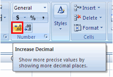
o Click once on the Increase Decimal button on the Home toolbar.

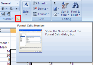
o The other way of adding decimals is to click on the number menu arrow as shown below to bring up the Format Cells window.

o Under Category choose percentage then you can set the number of decimal places.

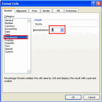
· In this window, the data can be formatted to look like currency with a $, or like percentages with a %. The results of our formulas or any other data can be formatted on our sheet to look like any type of data by selecting a different Category and setting different options.

5. Create a column to calculate the overall final mark for each student.

6. In the column to the right of the Final Exam Percent column enter the column header “Final Mark”

7. Create a formula to calculate students’ final weighted mark.

Note: This will be a long formula which will require you to multiply the percent for each student by the weighted value (found below the marked out of value). For example =(D5*C$33) can be used to determine the weighted value for assignment 1.

You will then have to add that to the weighted values for Assignment 2 and so on to determine the overall final mark. For example =(D5*C$33)+(assignment 2 percent * weighted value) etc… Remember you will have to use absolute referencing in order to copy the formula down so that it works for all students).

8. Format the results for each student’s final mark to be displayed in percent and to include one decimal place e.g. (65.4% not 0.654).

9. Create a new column to display if students received honours or not.

10.In the column to the right of the Final Mark column enter the column header “Honours”

11.Insert a formula that will display an “H” in the “Honours” column if the student got a final mark that is equal to 80% or higher and will display an “R” if they did not get a mark over 80%

12.(Hint: you will want to use the “IF” function” to do this and you will want to ensure that a mark of exactly 80% receives honours)

Some helpful symbols for you:

> greater than

< less than

>= greater than or equal to

<= less than or equal to

· If you have never used functions within Excel, it is recommended at this point that you go to the Functions section of your Prep Sheet read up on them.

· To insert a function into a cell, click on the cell where you want to see the result, then click on the Formulas tab, then click on the Insert Function button.

· Choose the desired function, and click OK. If you can’t find the function you are looking for select the All category and you will see all functions listed in alphabetical order.

· Your current assignment makes use of the "IF" function, specifically to determine whether or not students will receive honours.

· The "IF" function is referred to as a conditional function.  A conditional function can return different results based on a certain condition being evaluated to True or False. 

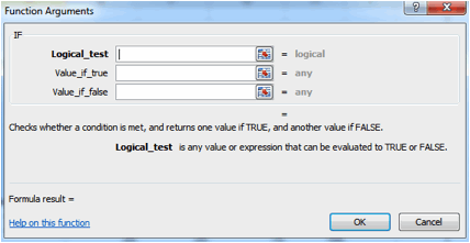
· The "Logical_test" text box shown in the above screenshot is where you type the condition that will be evaluated.

· So if that condition proves to be True we can get it to return a certain result, and if that condition proves to be False then we can get it to return a different result.

· What is being tested in the lab is whether or not a student received a final grade over 80%. If they did we want to display a value of “H” and if false we want it to display a value of “R”.

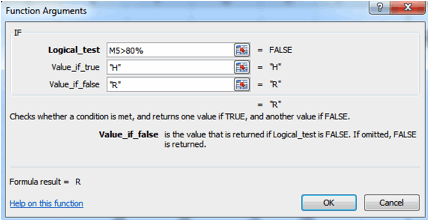
· In the example shown above it is returning the value of FALSE, which means that the value in cell M5 is less than 80%. So on the spreadsheet the letter R will be displayed.

· If the value in cell M5 was greater than 80% then the condition would be evaluated as True, and the letter H would be displayed.

13.Sort the students on your spreadsheet in ascending according to their ID number.

Note: be sure that the students’ data gets sorted along with the ID numbers, otherwise you will mix up which marks go with which student

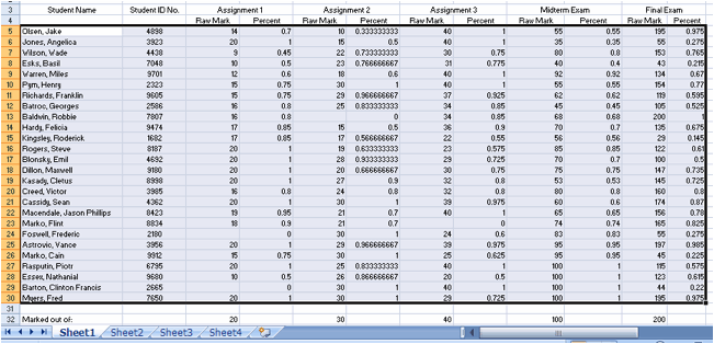
· First, indicate which data in the spreadsheet is to be sorted. Select the range of data you want to sort, making sure that all the data you want to move as a result of the sort has been selected as shown below:

Note: No column headings are selected just the data that will be shifted as the result of the sort

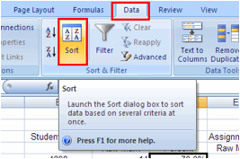
· Select the Data tab and click on the Sort button.

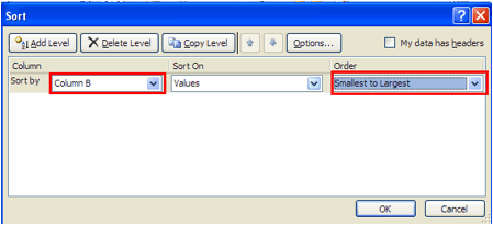
· The Sort options window appears. Choose the column you wish to sort by (in this case it is the column with the ID number, column B) and then choose the order you wish to sort by either Largest to Smallest, or Smallest to Largest. Once you have the right options click on OK.

14.Bold the main title and change the font and size to Arial 24. Merge and Center the title across all of the columns containing data in the spreadsheet.

15.Bold the individual column headings as well, and merge and center them across the two columns for each assignment and exam (raw mark and percent).

· To format the data on your sheet there are a few different options. First, select the cell or range of cells you want to format.

· You can use the available buttons on the Home tab.

· You can also select the Format drop-down menu from the Cells section of the Home tab.

· Select Format Cells.

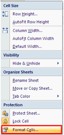
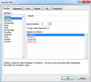
· The Format Cells menu will appear giving you many options to formatting your text.

· Merging cells is where you take a range of cells and merge them together as if they are one cell. An example of merged cells is shown below. Cells A1 through H1 of a sheet are merged (treated as if they were one cell), and the text is also centered within this larger cell area.

· To merge data we first need to select the cells we want to merge. Start by clicking on the cell which contains the content you wish to keep. Then continue selected the range of cells you wish to merge into one.

· Then with the cells highlighted, use the Merge and Center button found on the formatting toolbar.

16. Format the borders around all cells so that there is a thin border around all cells as shown below:

· To set borders, first select the range of cells around which you want to put borders.

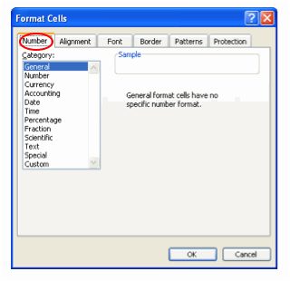
· ow select the Border tab from the Format Cells menu.

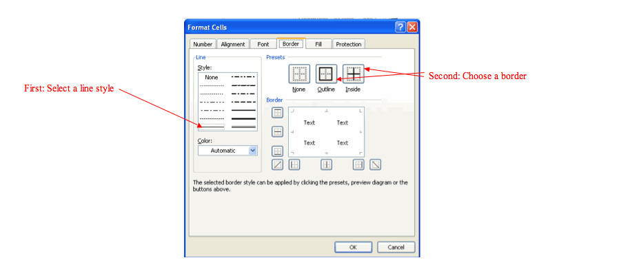
· To select your borders you first select the line style. With the current line style selected, click on the border you wish to apply it to within the border display box. Continue this process until all your borders are created.

17. Insert Cell Comments (as listed below in “ ”) into the following cells

· Cell C3 (Assignment 1): “Statistics Project”

· Cell E3 (Assignment 2): “Finance Project”

· Cell G3 (Assignment 3): “Design Project”

· Cell N3 (Honours): “H = honours R = regular Honours is awarded to a final mark of 80% or higher”

· To add a comment to a cell, right click on the cell to which you want to add the comment and select Insert Comment from the available context menu.

· In the comment box, type your comment text. When you finish typing the text you can single click on the edge of the box to place it in a different location. When you are happy with the placement, single click outside the comment box.

· Wherever the comment box is placed will be where it will appear when you drag your mouse over the cell that has the comment.

· To edit an existing cell comment, once again right click on the cell with the comment you want to edit, and select Edit Comment from the context menu.

18. Rename this worksheet “Student Marks”.

· An Excel document is called a “workbook”. A workbook can contain many “worksheets”. What you have been currently working on is one worksheet (currently named Sheet 1) within your LABSEC-CCID-SpreadSheet.xlsx file.

· If you look at the bottom-left portion of the Excel program window you will see the following navigation arrows and tabs:

· The tabs represent worksheets; the bolded tab is the worksheet you are currently looking at. You can navigate between worksheets by clicking on the tabs.

· To rename an Excel worksheet right-click on the worksheet tab at the bottom of the screen and choose “Rename” from the context menu, then type in the new name.

· At this point it would be useful to compare your “Student Marks” worksheet with the same worksheet in the sample file (linked on the WebCT assignment page).

· You’ll want to particularly scrutinize the results of your formulas and verify all the numbers match up. (In a real-world scenario, you would have to do this verification against some numbers you calculate yourself by hand or calculator)

19. Start work on Sheet 2 and name it “Assessment Statistics”

20. Inside the “Assessment Statistics” worksheet, you should see the following information:

21. Format column and row headers to be bold

22. Format borders: thin borders inside.

23.In the row titled “Class Average” insert functions that calculate the average mark for each assignment and exam. Format the results to display in percent with one decimal place. For this one we recommend the AVERAGE function

· Inserting these functions is the same process as you have done previously. The only difference is that you will have to reference cells on a different worksheet.

· When you wish to reference a cell or cells from another worksheet select the desired worksheet and then click on the cells you wish to reference. You will notice that the cell information will automatically be inserted into your formula or function.

24. In the row titled “50% and below” insert functions that calculate the number of marks below 50% for each assignment and exam. For this one we recommend the COUNTIF function.

· If you can’t find the COUNTIF function, change the category to All and search for it alphabetically.

25. In the row titled “90% and above” insert functions that calculate the number of marks above 90% for each assignment and exam. For this one we recommend the COUNTIF function.

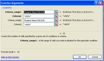
26. In the row titled “Between 50% and 90%” create a formula that calculates the number of marks between 50% and up to 90%. For this one we recommend the COUNTIFS function to select two ranges and the two different criteria as the COUNTIF function will not be able to evaluate two criteria at once.

27. Insert a pie chart in the “Assessment Statistics” worksheet that compares the number of students within the 3 different ranges of marks for the Final Exam (50% and below, 90% and above, Between 50% and 90%).

· chart title: Final Exam Analysis

· insert as object within the worksheet

· To create a chart in Excel first select the cells that contain the data that you want to appear in the chart. If you want column and row labels to appear in the chart, include the cells that contain them in the selection.

· To select more than one range of data, click and drag to select one range, and make sure it is highlighted. Then hold down the CTRL key on your keyboard and click and drag to select the next range of data.

· For our assignment the cells to select would look like this:

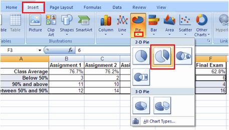
· Once you have your data ranges selected, click to select the Insert tab and then click on the Pie down menu to select a type of pie chart.

· This will add the following chart to your page.

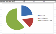
· To add a title to your chart you will first have to pick a chart layout that has a chart title. To choose a different chart layout single click to select the chart while it’s on the sheet and you should see the following menu options.

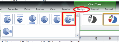
a) Single click on the Chart Layouts drop down menu to select a different chart layout.

b) Select a chart layout until find one with a title and legend (Layout 6).

c) To change the chart title single click on the Chart Title box and type in the following title and hit Enter.

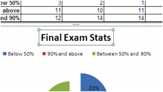
28. Create a line chart that tracks the class averages for all assignments and exams and meets the following criteria:

· marks data is along the Y-axis and that the range is 0% - 100%

· X-axis labels: the assignment descriptions

· Chart Title: Class Average

· Chart created on a separate sheet labeled “Student Marks Chart” (you can specify this at Step 4 of the Chart Wizard).

· All other chart options can be added but are considered optional.

· The initial selection for this chart would look like this:

· Once you have your data ranges selected, click on the Insert tab and choose the following options.

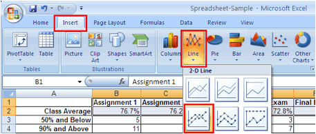
· The following chart should now appear on your sheet.

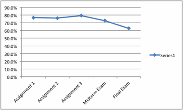
· As you have done with the previous chart click to select any available layout for your chart.

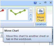
· To add the chart as a new sheet click on the Move Chart button located in the top right hand corner of the program interface.

· The following Move Chart window should appear:

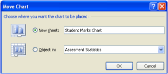
· Single click to select the New sheet radio button and type in the title Student Marks Chart and click on OK. This will add a new sheet to your workbook

· To change the percentage scale on your page so that it reaches %100 percent right click anywhere along the Y-Axis and select Format Axis as shown below.

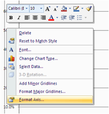
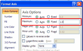
· This will cause the Format Axis window to appear. Under the Axis Options change the Maximum to Fixed value to 1.0 and click on Close.

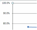
· Your percentage scale should now appear as %100.

· Now we add a data label to your series so that it says Class Average and not just Series 1.

· With your chart open single click to select the Select Data button.

· The Select Data Source window will appear.

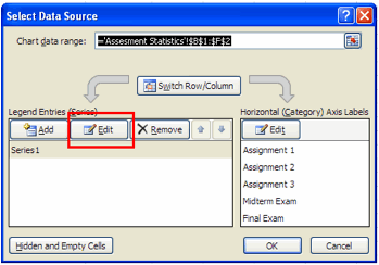
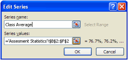
· Single click to select the Edit button and the following Edit Series window will appear. Type in Class Average for the Series name and click on OK.

· Click on OK in the Select Data Source window and the series name should now appear as Class Average.

29.Apply conditional formatting to your Student Marks worksheet so that any instances where a student has no grade for a particular assignment or exam is indicated by a red background cell color.

In Excel conditional formatting means to format a specific cell or range of cells a certain way if it meets a certain condition. For example in a given range of cells we can choose to format cells whose value is greater than 10 to appear bold and italicized.

· To apply conditional formatting to your sheet first select the entire range of raw data (no column headings as shown below) on your Student Marks sheet.

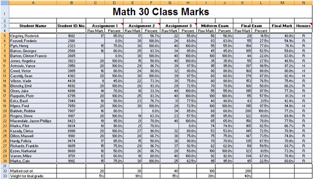
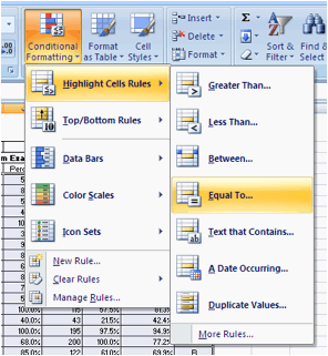
· Your next step is to select the Home tab on your toolbar and click on the Conditional Formatting button and choose the options as shown below. We are choosing the Equal to value because we want to format all the cells that are equal to 0. Based on what you would want to find you would choose different options such as Greater Than or Less Than:

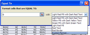
· This will bring up the following Equal To window. Using this window we will be able to format all cells that are equal to 0 to have a red background color.

· Type in 0 as your EQUAL TO: value and from the with drop down menu choose Custom Format…

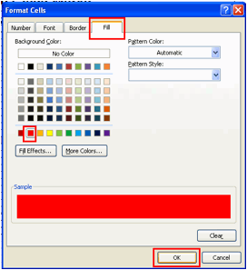
· This will open the Format Cells window. Click on the Fill tab, single click on a red background color, and click on OK.

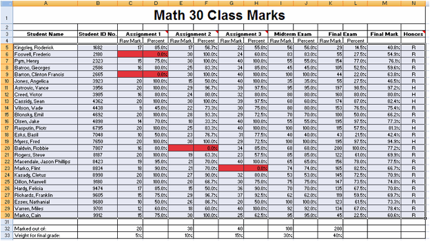
· Click on OK in the Equal To window and you should now see all empty cells where students did not complete an assignment formatted with a dark red background color.

30. Include a column in your spreadsheet that will display a student’s letter grade based on their Final Mark. When determining your formula, be sure to include cell references rather than just numerical values. For example, your formula should read “=IF(A1>B42)” not “=IF(A1>90%)”.

· One column to the right of the “Honours” column type in the heading “Letter Grade”.

· The letter grade formula is a complex formula that will require the use of a nested “IF” function and will require it to be typed in without using the function wizard. For this function we are going start by using the Help menu. Once in the help menu we can copy and paste the sample formula for the nested “IF” function included in the Help Menu.

· Once we have copied and paste the function all that remains is to replace the sample cell values with the values that are on our Student Marks sheet.

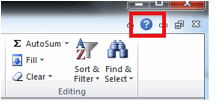
· To begin using the help menu click on the Help Menu icon in the upper right hand corner of the program interface as shown below.

· This should bring up the following Excel Help menu. Type in IF into search field entry box and click on Search.

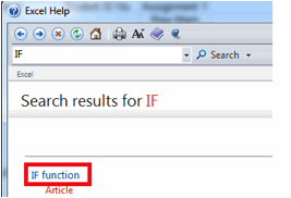
· This will display the following search results. Click on the IF function link.

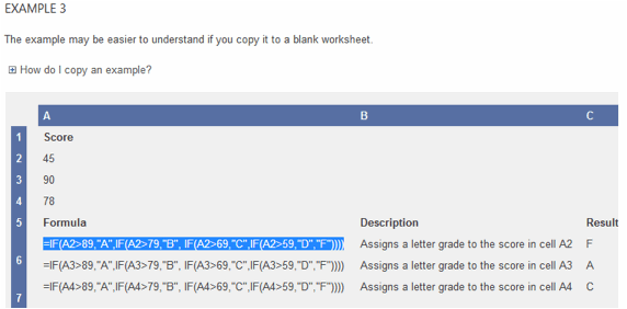
· This will bring up in IF function help page. Read over the available information and refer to Example 3 which gives a detailed description on how to insert the nested IF function

· Copy and paste one of the formulas used in Example 3 into your spreadsheet and replace the cell values they used with the ones on your sheet.

· Use the following guidelines to replace the cell values so the function will work with your sheet:

o Edit all your final mark values to refer to cell M5 and not cell A2.

o Replace the sample cutoff values with the following values:

§ A would be equal to or greater than 85%

§ B would be equal to or greater than 75%

§ C would be equal to or greater than 65%

§ D would be equal to or greater than 55%

§ F would be less than 55%

Note: Be sure to include the percent symbols ( % ) for your cutoff values.

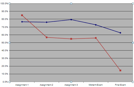
31. Add a new student data series to your existing line chart, Student Marks Chart.

Currently the Student Marks Chart only displays the average results of the entire class. What if you wanted to modify your chart so that you can compare one student to the overall class average?

· To add another series of data to an existing chart you first have to click on the Student Marks Chart tab.

· Click to select the Design tab and then to add more data click on the Select Data button

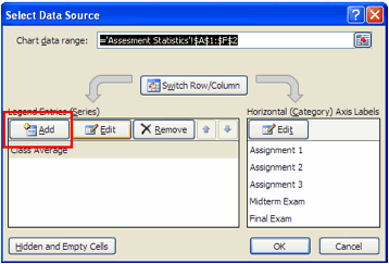
· This will open the Assessment Statistics page and open the Select Data Source window. Click on the Add button to add another series of data to your chart.

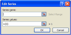
· This will open the Edit Series window as shown below. We told Excel that we want to add more data now we have to select that data.

· To select the data click on the Student Marks tab and single click to select one of the students on the sheet. (Make sure you click in the Series name field before selecting the student).

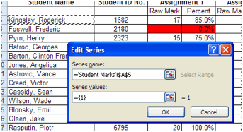
Notice that the name is not typed into the Series name field but the cell reference.

· For the Series values first delete the existing text.

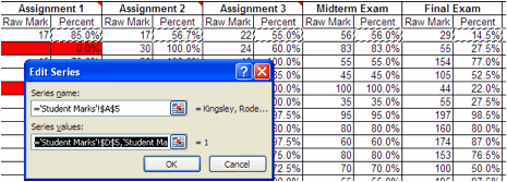
· Then once again click on the Student Marks tab and using the CTRL key select the individual percentage values for all assignments and exams. You will see the corresponding cell references appear in the Series values field.

· Once you have selected all the correct data click on OK, click on OK in the Select Data Source window and you should see the new data series for your chosen student added to your chart.

32. Modify your Student Marks worksheet so that only the cells with Raw Data (ie. Student Name, Student ID, Raw Marks for all assignments and exams) can be modified or have data entered into them when the sheet is protected.

· First select the ranges of data on the sheet you want to be able to edit after the entire worksheet has been protected. Single click on the Home tab and select the following options from the Format cells menu.

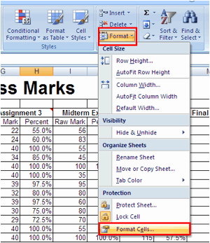
· The Format Cells window should appear. Click on the Protection tab. Click in the box next to Locked to remove the check mark. Click OK. You have now set the Locked property for these cells to false. In other words you have unlocked these cells.

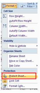
· Our next step is to protect our entire worksheet. From the same Home tab click on the Format drop down menu and select Protect Sheet….

· The Protect Sheet window appears. Leave the options as they are and click OK. This ensures that every object on your sheet, aside from the ranges of cells you unlocked, will be unchangeable after the sheet has been protected.

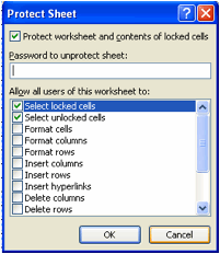
· To protect other objects or set options on your sheet, single click to add a checkmark in the above check boxes.

· You also have the option to assign a password. This way only the people that know the password will be able to unprotect the worksheet and make changes. However, if you are ever submitting a spreadsheet for marking you do not want to set a password. The person marking your sheet will need to unprotect it in order mark it.

· Now if you try to alter the contents of any of the locked cells, you will not be able to. You should, however, be able to modify the data in the unlocked cells.

· If you want to change the locked property of cells, the worksheet must be unprotected. Thus, once you have protected a sheet, you must unprotect it before you can modify the locked settings or any other settings.

· To remove protection from a worksheet, select Protection > Unprotect Sheet from the Tools menu. If you entered a password, you will be prompted to enter the protection password for the worksheet.

· To move between unlocked cells on a protected worksheet, click an unlocked cell, and then press the Tab key. The Tab key is a handy way to let you cycle through the unlocked cells of a sheet.

33.Submit your “LABSEC-CCID-SpreadSheet.xlsx” file in Moodle.

---

Steven Scott & Jeff Warner

University of Alberta