May - August 2006,
Department of Mathematical and Statistical Sciences, University of Alberta
|
|
|
Research performed by Amenda Chow and Tyler Pittman, May - August 2006, Department of Mathematical and Statistical Sciences, University of Alberta |
The partially mixed region is an isolated uniformly dense area in a stratified fluid much like the oil spill or toxic gas in the ocean or atmosphere, respectively. The movement of this mixed region through the stratified fluid is known as an intrusion. Our main focus is how this intrusion affects the ambience. We concentrate heavily on how the internal waves created by the intrusion disturb the stratified fluid. Results from this can help environmentalists determine how fast the oil spill spreads or how long it takes for the toxic gas to become harmless.
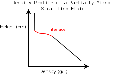
After the tank is filled and ample time is given for the stratified fluid to settle, a conductivity probe traverses vertically through the tank providing us with a density profile of our uniformly stratified fluid.
A gate is inserted inside the tank 18.5cm from the edge to the bottom of the mixed region and this section of the tank is now known as the lock. The gate acts as a barrier preventing fluid from entering the lock. By lowering the gate only to the bottom of the mixed region, this reduces the waves caused by the pulling of the gate and allows us to be confident that the waves created below the mixed region is a result of only the intrusion.
A square screen of horizontal black and white lines is placed behind the tank just after the lock. The screen is required for synthetic schlieren. This digital image process records the distortion of the image of horizontal lines due to the bending of light through various density gradients.
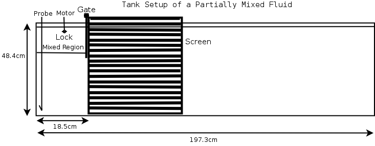
At the lock we place our electric motor 1cm from the surface of the fluid and mix a uniform region of desired height (in this case, heights of 5, 10, 15cm are created). We make another traverse with our conductivity probe and then wait for the tank to settle before releasing the gate.
While waiting for the tank to settle, we setup our camera. Each experiment is recorded from just before release of the gate until the tank settles using a digital camera placed 300cm in front of the screen. The recording is digitized and analyzed using the image processing program, DigImage.
Most of our analysis is done on DigImage which is specifically designed for analyzing fluid flows. One of its features is it can create horizontal time series (HTS) (see Results to view actual HTS images) of the intrusion as it moves along the tank. Using the HTS, we calculated useful characteristics of the intrusion such as intrusion speed.
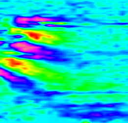
DigImage also creates false colour processed vertical time series (VTS) images called DNT images (see Results to view actual DNT images) which represents the change of the buoyancy frequency (N) squared. DNT images illustrate the movement of wave packets created by the intrusion with respect to time. They visually enhance the internal waves created by the intrusion and allow us to identify crests and troughs, as well as determining the wavelength. We also made approximations on wave properties such as N2t (range) and vertical displacement (amplitude) using these DNT images.
As well, we took horizontal slices from stored VTS and DNT files, translated them vertically and interpolated the gaps between each slice to come up with an image in x,t coordinates. These xtdnt images allow us to calculate the speed of the wave packets (horizontal phase speed).
Aside from using DigImage, we also investigated the density profiles of our stratified fluid (see diagram at right). We determined a piece-wise function to approximate the density profiles and modified code in the C language that calculated the thickness of the interface and the mean depth of the interface. We also determined the slope of our density profiles which we needed for N and collaspe time of our intrusion.
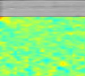
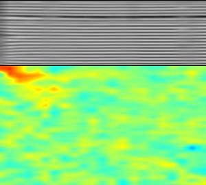
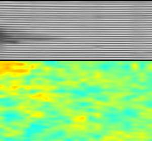
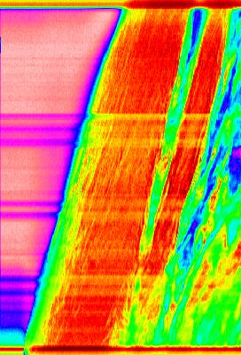
Here we have chosen 3 movies illustrating the release of a partially mixed region in a stratified fluid. The fixed parameters of the associated experiments are: rhoBottom~1.10g/L and lock=18.5cm. The movies are split into two screens, the upper part (black & white) is the raw image of the experiment corresponding to the intrusion of the partially mixed region and the lower part (colour) is the processed image data representing the wave packets.
| Duration=30sec | Duration=30sec | Duration=30sec |
|---|---|---|
| Length=30.0cm | Length=30.0cm | Length=30.0cm |
| Height (B & W)=5.8cm | Height (B & W)=9.5cm | Height (B & W)=12.0cm |
| Height (Colour)=21.0cm | Height (Colour)=17.5cm | Height (Colour)=16.0cm |
| video of 5cm mixed region | video of 10cm mixed region | video of 15cm mixed region |
|
|
|
Using horizontal time series images (here in false colour), we calculated the speed and observed that as the height of mixed region increases, the greater its speed.
| Time (vert. axis):~34sec | Time (vert. axis):~34sec | Time (vert. axis):~34sec |
|---|---|---|
| Distance (horiz. axis):~33.0cm | Distance (horiz. axis):~33.0cm | Distance (horiz. axis):~33.7cm |
| Horiz. time series at z=30.9cm | Horiz. time series at z=27.9cm | Horiz. time series at z=27.2cm |
|
|
|
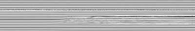
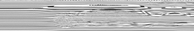
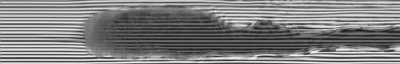
These vertical time series are taken from actual images of the experiment.
| Time (horiz. axis):~34sec | Time (horiz. axis):~34sec | Time (horiz. axis):~34sec |
|---|---|---|
| Height (vert. axis):~5.0cm | Height (vert. axis):~10.0cm | Height (vert. axis):~15.0cm |
| Vert. time series at x=13.6cm | Vert. time series at x=13.6cm | Vert. time series at x=13.3cm |
|
|
|
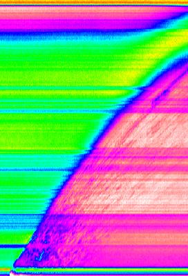
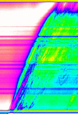
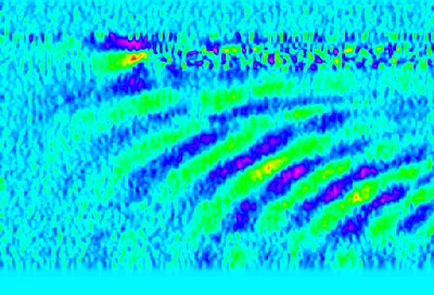
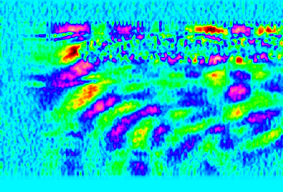
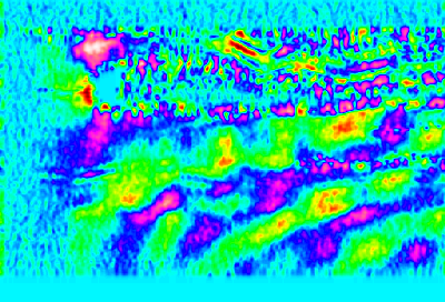
Using the DNT images (contours of the time derivative of the perturbation squared buoyancy frequency), we measured the period of the waves and observed that as the height of the mixed region increases, the period also increases.
| Time (horiz. axis):~34sec | Time (horiz. axis):~34sec | Time (horiz. axis):~34sec |
|---|---|---|
| Height (vert. axis):~30cm | Height (vert. axis):~30cm | Height (vert. axis):~30cm |
| Vert. TS of DNT at 13.6cm | Vert. TS of DNT at 13.6cm | Vert. TS of DNT at 13.3cm |
|
|
|
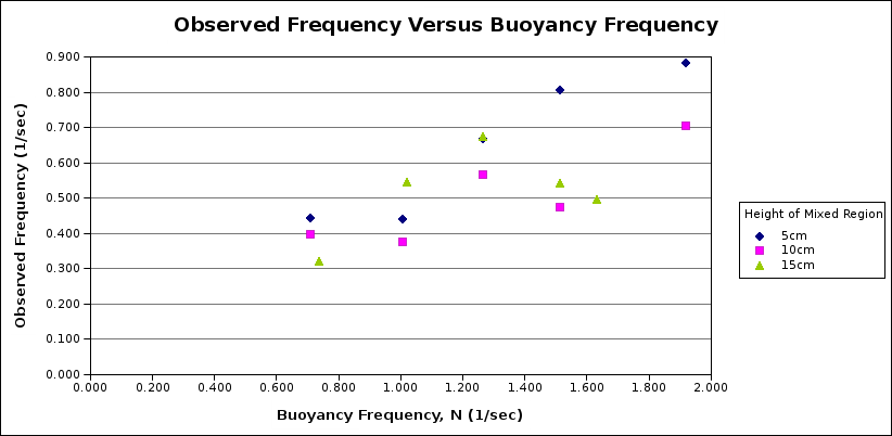
| Associated values for Plot | |||
| RhoBottom (g/L) | Height of Intrusion | Buoyancy Frequency (N) | Observed Frequency |
| (cm) | (1/sec) | (1/sec) | |
| 1.02 | 5 | 0.708 | 0.442 |
| 1.02 | 10 | 0.708 | 0.398 |
| 1.02 | 15 | 0.738 | 0.321 |
| 1.04 | 5 | 1.005 | 0.439 |
| 1.04 | 10 | 1.005 | 0.376 |
| 1.04 | 15 | 1.019 | 0.546 |
| 1.06 | 5 | 1.264 | 0.668 |
| 1.06 | 10 | 1.264 | 0.566 |
| 1.06 | 15 | 1.264 | 0.676 |
| 1.08 | 5 | 1.514 | 0.806 |
| 1.08 | 10 | 1.514 | 0.476 |
| 1.08 | 15 | 1.514 | 0.542 |
| 1.10 | 5 | 1.920 | 0.885 |
| 1.10 | 10 | 1.920 | 0.706 |
| 1.10 | 15 | 1.633 | 0.495 |
From the above plot and corresponding table of values, we make several observations. Clearly, as rhoBottom increases, N increases, which implies the period of the waves descreases. Buoyancy frequency appears to exceed the observed frequency for all the experiments. There is no strong evidence suggesting that a larger mixed region has an effect on either frequency.
Department of Earth and Atmospheric Sciences