May - August 2005,
Department of Mathematical and Statistical Sciences, University of Alberta
|
|
|
Research performed by Cara Kozack, May - August 2005, Department of Mathematical and Statistical Sciences, University of Alberta |
|
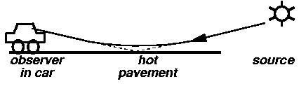
The phenomenon of light bending as it travels though a density changing fluid is a common and often observed phenomenon. While you are traveling along the highway on a hot day, often you can see the image of water on the highway. This is due to the light rays being bent through the different layers of air (see image right). There is a mathematical relation between how much the light bends and how quickly the density changes in the fluid. The formula is based on the geometry of how the light passes through the medium (straight line, at an angle) as well as the amounts of different material it passes through (water bends light more than air, so if the light beam passes through more water the light will be bent more). If you know how much the density changes you can plug this value into the formula and calculate the displacement of the light ray. However, the amount the light bends is a measurable quantity, the density often is not, especially in a chaotic environment. In a controlled experiment using a synthetic schlieren with light traveling through a stratified fluid, this bending can be measured and the change in density calculated from the inverse of the geometric formula.
|
 |
|
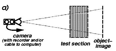
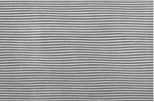
Taking the setup to the left (described in detail in Dalziel, Hughes, Sutherland (2000)) snapshots of 'object-image' are taken. One before the density of the tank changes, and while the density is changing from some sort of disturbance (like bobbing a ball up and down). The appearance of the image becomes distorted due to the light coming from it being bent in the water. Light travels from the object, through the tank, to the camera which is able to record the changes over time. Then the difference between the initial image and the distorted image is computed; this represents where, and how much the light has been bent while going through the fluid |
|
|
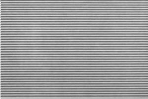
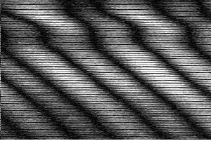
| The initial grid lines in the camera's field of view, with the light rays traveling straight through the test material. | Once the tank has been disturbed another image is taken, the lines are slightly wavey because the light returning to the camera has been bent by the change of density in the tank. |
|
|
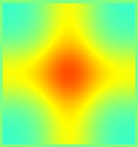
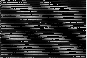
| The difference between the first and 2nd images. The greatest change in the relative position of the lines shows up very obviously in this image - which represents where the density had changed the most between the two times. | A graphical representation of exact numerical value of how much the fluid was distorted can be gleaned from the difference image. By computing the intensity of the difference and putting it into the inverse formula for the change in density. |
The above research is somewhat simplified since it only requires a formula for a plane (see also Sutherland, Dalziel, Hughes, Linden (2000)). If the disturbance is 3 dimensional the formula to calculate the change in density is much more complicated and is generally not possible to invert exactly. Previous research had been done to create a 2 perspective problem in which two perpendicular camera views are used. This solution had an asymmetry which resulted in 2 "bars" extending from the final solution. My initial task for this project involved taking that method and creating one that used four camera views in the hopes that it would recreate a test density profile.
The experiment that this project hoped to get a mathematical framework for is towing a sphere through a stratified fluid to generate internal waves. In this problem the fluid displacement delta-z is measured and delta-N2 the buoyancy frequency) needs to be calculated. The relation for this problem is delta-z = G*delta-N2 where G is a geometric representation of the path that light takes on its traversal through the tank to the camera. G is constructed based on the distances from the camera to the tank as well as the index of refraction (the measure of how much light bends) of light in salt water, air, and perspex
The equations for solving a 3D problem like this are such that there is not a unique solution to the problem; for a resolution of n there are 4*n equations and n2 unknowns. This gives the problem that the solutions that are obtained are not necessarily the solutions that correctly represent the physical situation. Not only is G a difficult function to invert it also can be tricky to pinpoint the correct way to invert it to give a reasonable answer.
This project involves solving a 3 dimensional tomography problem using mathematical inversion techniques. With tomography we can reconstruct delta-N2 using G and the measured delta-z. In general, a "map" of a characteristic variable can be obtained as long as you can measure something that has a relation to that variable and you know the relation. In general if you want X, you can measure Y and you know X = F(Y) where F is some function, then you can collect values of Y and calculate X. However if you want Y but can only measure X then you need to find an inverse of F. In many cases F is too complicated for regular inversion methods. Inverse tomography helps to calculate our wanted quantity by using tricks to find some way to use what we know to find something that represents that inverse.
This technique is used in medical imaging for CT scans as well as in geophysics for reconstructing models of the earth from seismic imaging
For a tomography problem that has symmetry only one dimension is needed to obtain a full set of information about the situation. For a problem that is lacking in symmetry, information from additional perspectives are needed to resolve the full solution. Adding these extra perspective is the method I will use solve this inverse tomography problem. It is hoped that the extra information from the other points of view will be enough so that the problem has a solution that is close to the one that is wanted
The mathematical setup of this problem is that of a discritized matrix problem of the formula

Where delta-z and delta-N2 are vectors and G is the matrix. For a resolution of n delta-N2 is a vector of length n2, that represents a single slice of the tank that is nxn unwrapped into a single matrix. The vector delta-z has a length of np, where p is the number of perspectives used. Each sub-vector of delta-z (of length n) represents the displacement the camera sees along the tank wall at a particular vertical slice.
My first attempt at the problem involved calculating the pseudo-inverse of G. That is, a function that I could multiply delta-z by and get delta-N2.
The mathematical method for calculating the inverse is as follows
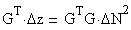
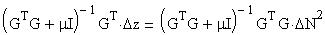
Where the term multiplying both sides in the 2nd equation is the pseudo-inverse. The 2nd term in the pseudo-inverse is known as a preconditioning parameter. G times G transpose is very sparse with only 1/n3 entries being non-zero. The LU decomposition routine makes this matrix into a lower and upper triangular matrix, but its singular. This problem can be avoided by adding a preconditioning matrix to GTG so there are non-zero entries on the diagonal. The preconditioning parameter mu multiplies the identity. In both the computation of the rectangular coordinate pseudo-inverse and the polar coordinate pseudo inverse the value of mu was kept at 0.00001. This value was chosen because anything smaller didn't lead to any better results and any value that was larger tended to smear out the solution structure.
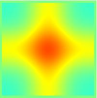
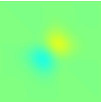
I used a 2D symmetric Gaussian hump (a bell curve) as my test delta-N2 to calculate a set of delta-z profiles exactly in a forward problem. I could then take these delta-z profiles and check to see if my inversion routine would return the original delta-N2. Shown below are the results for 3 and 4 cameras with a fairly low resolution of only 20 grid points per side. The actual problem would use close to 512 but the time to run the program for much more than 20 increases as 4*n9 at least. The time to run a resolution of 20 (the matrix G then being 80x400) on a SGI machine took about 30 seconds.
|
|

|
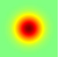
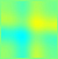
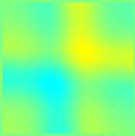
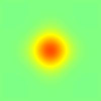
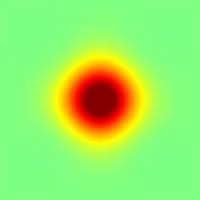
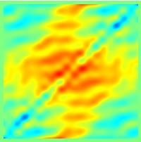
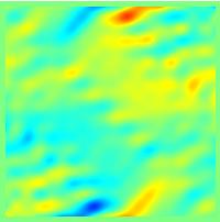
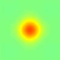
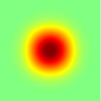
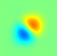
| The original gaussian profile as a 2D contour plot. In all the below pictures involving delta-N2 being a gaussian the desired result is this. | Gaussian profile with 3 cameras | Gaussian profile with 4 cameras |
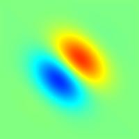
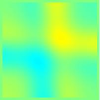
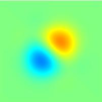
The cross pattern that emerges seems to be an artifact of the inversion process, no matter of size, shape, amplitude, or location of the delta-N2 disturbance, perpendicular bars emerged. Below is another set of images for 3 and 4 cameras with a different test profile of a gaussian*sin.
|
|
|
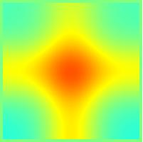
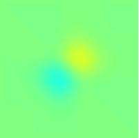
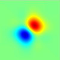
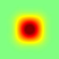
| The original sin*gaussian profile as a 2D contour plot. In all the below pictures involving delta-N2 being a sin*gaussian the desired result is this. | Sin*Gaussian profile with 3 cameras | Sin*Gaussian profile with 4 cameras |
In an attempt to put the solution more towards the center I tried multiplying my final solution with a gaussian weight. Data near the center would get a larger amplitude and the data near the edges would be smaller. This is what it looks like for both the gaussian and the gaussian-sin. The disadvantage of this method is that it depends on what the delta-N2 profiles looks like, this apriori knowledge is not always available and in some cases may give a false sense of the accuracy of the solution. Although it may happen that the gaussian weight is general enough for any weight.
|
|
|
|
|
|
|
Original Profile |
Original Profile |
Gaussian profile, 4 cameras, weighted | Sin* Gaussian profile, 4 cameras, weighted | Gaussian profile, 4 cameras, weighted with a double amplitude gaussian | Sin*Gaussian profile, 4 cameras, weighted with a 5X amplitude gaussian |
This seemed to get rid of the symmetry, but at a cost to the amplitude. This suggests that the inversion technique was flawed in some way, it was returning a solution, but it was not converging in the way that was necessary. A better solution would have stayed in the center and retained its axisymmetric symmetry rather than its 4 way symmetry. Making a larger amplitude weight seemed to fix the amplitude problem, but not enough for the sin*gaussian profile. Increasing the amplitude further showed the reappearance of the 4 fold symmetry and the method seems mathematically artificial
A possible solution to this problem would be to switch from Cartesian coordinates to a polar coordinate system. G and delta-N2 previously were defined on a square grid, with the tank area divided into equal area segments. In polar coordinates the tank ares would be divided into circles and radial lines, intersecting at the center of the tank. This would increase the number of grid areas in the center of the tank, as well as increasing the resolution there.
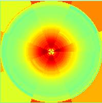
After this was implemented I tried using just circles on the axisymmetric gaussian profile. Below are the results using a high resolution(100 circles 100 grid points to a side taking almost no time to run) with 1 and 4 cameras.
|
|
|
|
Original Profile |
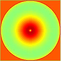
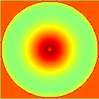
Gaussian profile pseudo-inverse using polar coordinates with 1 camera, (only circles in geometry | Gaussian profile pseudo-inverse using polar coordinates with 4 cameras (only circles in geometric setup) |
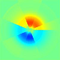
The results looked very promising with no sign of the four-fold symmetry as well as proper contour levels. Next I tried the gaussian profile with a few sectors using 1 and 4 cameras. The four fold symmetry reappeared, and the inversion technique ran much too long with even a low resolution of sectors (128 grid points, 64 circles, 8 sectors takes over 3 minutes and increases as (n*circles*sectors)3). However when the tests were repeated with the gaussian*sin profile, the results were a bit more promising. The symmetry was still present, but the results seemed much closer to the actual profile.
|
|
|
|
|
Original Profile |
Gaussian profile, 4 cameras, polar coordinates using both circles and sectors | Original Profile |
Sin* Gaussian profile, 4 cameras, polar coordinates using both circles and sectors |
Regardless of the results with the sectors the axisymmetric problem with only circles is very promising and this method can be used to solve axisymmetric synthetic schlieren problems (such as described in Onu, Flynn, Sutherland (2003)) fairly exactly and with minimal computational effort.
The final method I attempted to solve this problem with was the conjugate gradient method. This is an iterative solver that calculates a solution to some sparse linear problem through the use of residues and directional vectors. It's a much quicker method than the outright calculation of the pseudo inverse and there are several additional parameters that can be changed to increase the accuracy of the solution.
For an under determined problem such as the one we have, the CG method goes towards the minimum norm solution, that is that G*N2 - delta-z is as small as possible. But this isn't necessarily the best solution, so data weighting, model weighting, regularization, and preconditioning can be used to make the answer the one we want. These tweaks are chosen on a variety of test delta-N2 profiles, once the proper results are returned then it will be ready to go for a realistic set of delta-z data.
Running conjugate gradient without any of the options returns the following results for the gaussian and gaussian*sin. These are almost identical to the results for the pseudo-inverse with the advantage that it takes only a fraction of the time to run computationally. All the tests were done at 20 resolution but the resolution could be upped to 40 with only a slight increase in running time, which was close to instantaneous. This increase in speed was due to putting G in a sparse format which eliminated all the operations of multiplying by 0.
.|
|
|
|
|
Original Profile |
Conjugate gradient solution for gaussian profile | Original Profile |
Conjugate gradient solution for sin*gaussian profile |
Regularization is a form of "smoothing" the solution, which wasn't really necessary for this problem, but real data may be much more chaotic and rough. I tried smoothing using a first derivative, 2nd derivative, and a Laplacian. In reality the 1st and 2nd derivatives shouldn't have had any effect since the delta-N2 profile is in two dimensions. Indeed there was an asymmetry in the final output. The Laplacian didn't have that much asymmetry, but it was still not very much help in returning the wanted solution.
|
|
|
|
|
Original Profile |
Conjugate gradient solution for gaussian profile with a Laplacian smoothing regularization | Original Profile |
Conjugate gradient solution for sin*gaussian profile with a Laplacian smoothing regularization |
I didn't implement data weighting since the data I was using was smooth and error free, but I did implement model weighting in three ways in the code in a similar way to the gaussian weight for the Cartesian problem. First simply multiplying the resultant profile by the gaussian, next multiplying and then running CG again, and finally including the weight within the CG algorithm
|
|
|
|
|
Original Profile |
Conjugate gradient solution for gaussian profile with just weighting applied | Conjugate gradient solution for gaussian profile with weighting applied and then CG rerun | Conjugate gradient solution for gaussian profile with weighting included in CG routine |
|
|
|
|
|
Original Profile |
Conjugate gradient solution for sin*gaussian profile with just weighting applied | Conjugate gradient solution for sin*gaussian profile with weighting applied and then CG rerun | Conjugate gradient solution for sin*gaussian profile with weighting included in CG routine |
Inserting the weight after CG has the same effect as multiplying it after the pseudo-inverse routine. However including the weight as part of the CG routine not only gets rid of the symmetry but it is also more mathematically sound. The downside to this is that even though it works perfectly for the plain hump, it doesn't return the required amplitude for the sinusoidal one. This suggests that the hump works only in a specific case and doesn't correspond to a general fix.
A general fix for this problem is preconditioning. This is the process of changing the CG code so that it solves a matrix similar to the original one, but that has an easier to find solution. This is not a simple method to implement seeing as the preconditioning matrix must be the same size as the original set of equations, so it has the same problem of having more unknowns than equations. There are ways to find solutions to these types of problems, but it depends on the structure of the matrix. This preconditioning matrix is called such since it guides the CG algorithm towards the correct solution, but finding such a matrix can take a long time for each problem and so it is left to future research.
K. Onu, M.R. Flynn and B.R. Sutherland, Expt. Fluids,35,pp24-31 (2003).
S.B. Dalziel, G.O. Hughes and B.R. Sutherland, Expt. Fluids,28,pp322-325 (2000).
B.R. Sutherland, S.B. Dalziel, G.O. Hughes, P.F. Linden, J. Fluid Mech.,390,pp93-126 (2000).
Department of Earth and Atmospheric Sciences