As I wish to ideally derive a response function with more than one of the original variables, I first performed a PCA to find an optimized combination our variables. Then using a standard criteria I picked the principle components which capture the most variation in the data and retained those for the MR.
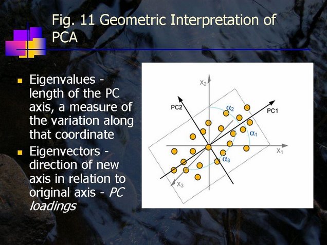
PCA rotates the coordinate space of our original variables such the longest axis (PC1) projects the most data. The length of the axis is referred to as its eigenvalue and is a measure of the variance in the data. Subsequent axis are made perpendicular to PC1 and explain progressively less and less of the variation in the data. The relationship between the new variables, or principle components, and their original variables is determined by their loadings. A higher loading means that the variable is more closely related to the principle component (Fig. 11). The PCA scores are the original data rotated into their new coordinate space.
At this point there are a number of criteria which can be used to reduce the number of principle component one carries into further analysis. The simplest, which is used in this example, is to discards those components with eigenvalues below 1. The outputs from the PCA analysis of monthly temperature and the first tree ring series are illustrated in Figs. 12 and 13.


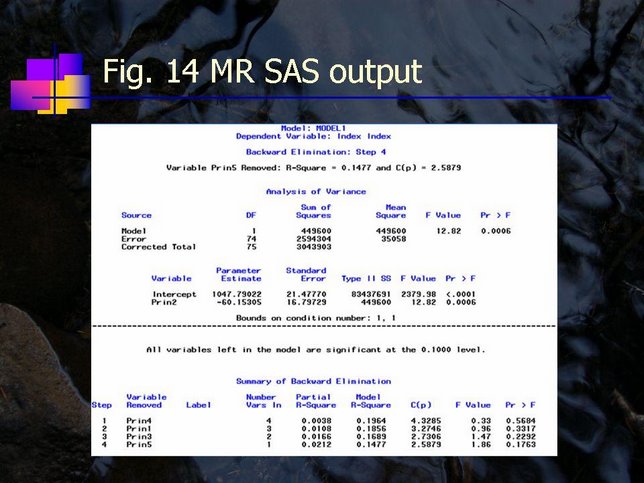
The eigenvalue one criteria suggests we should retain the first five principle components. Using the scores from these components we derive our model using MR. The MR discards all but the second principle component (Fig. 14).
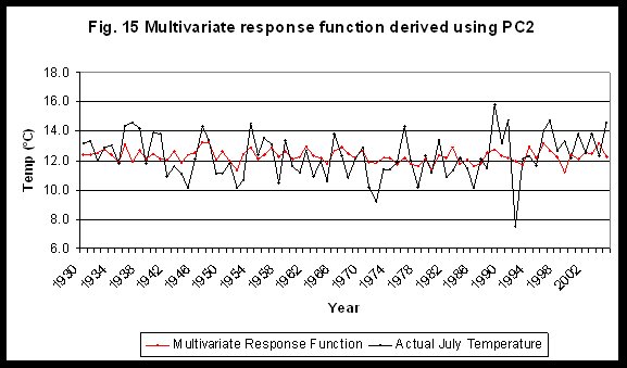
In this second component April and May temperatures are weighed highest (Fig. 13). Using our PC2 scores we calculate our July temperatures and derive our new response function (Fig. 15).