 PCA Biplots
The output links at the end of each section link to pages that show the applicable outputs from the program.
Select the images to view graphs/images outputted from the program.
The R Computing Program is a free statistical program that can be downloaded at the
R Website.
Look at the website for further information about the statistical computing program and other functions it can
preform.
The following function was written and run in R:
function (data,n) {

 id=seq(1,n,by=1.0)

 I=n*(sum(data[id]*(data[id]-1)))/((sum(data[id])*(sum(data[id])-1)))

 return(I)
}
To run this program the following code was used:
plotc.dat=read.table("C:/Laura's Documents/Renewable Resources/Ren501/Philippines Project/plotc.txt", header=T, blank.lines.skip=T)
c.almo=plotc.dat$species[plotc.dat$species=="almo"]
morisita.index.r(c.almo, 24)
Each species was entered into morisita.index.r separately for each stand. The n value (number of subplots sampled) entered for
the Young Growth (PLOTA) and Mid Growth (PLOTB) stands was 24 and the n value entered for the Old Growth stand (PLOTC) was 70.
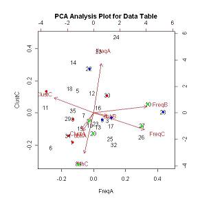
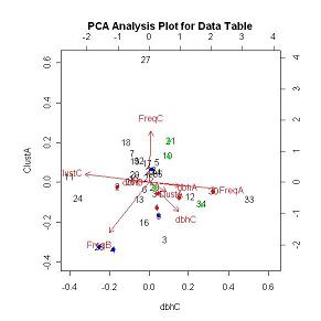
For the PCA Analysis the pre-written function princomp was used from the base package. The analysis could also be run using the pre-written function rda in the vegan package (syntax differs for this package).
The run the princomp function the follow code was used:

species.dat=read.table("C:/Laura's Documents/Renewable Resources/Ren501/Philippines Project/DataTable.txt", header=T, blank.lines.skip=T)
species.dat.pca=princomp(species.dat,cor=T)
To view the PCA scores the following code was used:

species.dat.pca$scores
Select the PCA Data Table link to view the PCA score generated from the PCA analysis for this project.
To view the PCA graph the following code was used:

biplot(species.dat.pca,choices=2:3)   (where choices determines which PCA component is graphed)
For the CLUSTER Analysis the following code in PROC CLUSTER was used:
PROC CLUSTER DATA=SPECIES METHOD=NORMAL OUTTREE=PLOTS;
   VAR FreqA FreqB FreqC ClustA ClustB ClustC dbhA dbhC;
RUN;

PROC TREE DATA=SPECIES;
RUN;
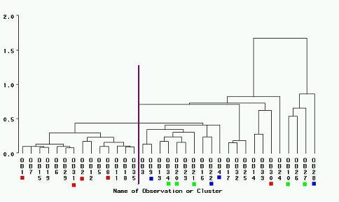 CLUSTER Dendrogram
PROC DISCRIM was used to calculate the F-statistics to test the difference amongst the group centroids for each successional classification, and predict the successional classification for the unknown species and to test the probability of incorrectly predicting a whether a species is an early, mid or late successional species. The following code was used to complete all 3 tasks:
PROC DISCRIM DATA=SPECIES TESTDATA=SPECIES METHOD=NORMAL POOL=YES OUT=SPECIES2 ALL;
   CLASS KNOWN;
   TESTCLASS KNOWN;
   VAR FreqA FreqB FreqC ClustA ClustB ClustC dbhA dbhC;
   PRIORS EQUAL;
RUN;
Select the F-Statistics link to view the F-statistics generated by the DISCRIM analysis for this project.
Select the Predicted Data Table link to view the differentiation results from the DISCRIM analysis.
Select the Error Percentages link to view the results from the misidentification test.
Select the DISCRIM Output link to view the entire results from the initial PROC DISCRIM analysis.
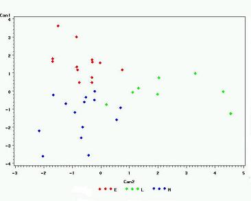
To view a graph of the differentiation between succession classification for the predicted and known species combined the following PROC CANDISK and PROC GPLOT code was used:
PROC CANDISK DATA=SPECIES2 OUT=SPECIES3;
   CLASS _INTO_;
   VAR FreqA FreqB FreqC ClustA ClustB ClustC dbhA dbhC;
RUN;

PROC GPLOT DATA=SPECIES3;
   PLOT CAN1*CAN2=KNOWN;
RUN;
 CANDISK Image
To analyze which variables significantly contributed to the successional classification of each species the following code in PROC STEPDISK was used:
PROC STEPDISK DATA=SPECIES2 METHOD=STEPwISE SLSTAY=0.15;
   CLASS _INTO_;
   VAR FreqA FreqB FreqC ClustA ClustB ClustC dbhA dbhC;
RUN;
Select the STEPWISE Output link to view the results from the stepwise selection.
HOME
INTRODUCTION
DATA DETAILS
MULTIVARIATE METHODS
MULTIVARIATE RESULTS & DISCUSSION
CONCLUSION
APPENDICES
REFERENCES & ACKNOWLEDGEMENTS
DATA PREPARATION METHODS
DATA PREPARATION RESULTS & DISCUSSION
PRELIMINARY ANALYSIS