 FIGURE 6
Since seed size and other life history trait variables that are typically used to determine whether a species is an early, mid or late successional species were not available in this data set, other variables needed to be generated from the data set to run an analysis.
Frequency of each species in each stand was a obvious variable to use because it was available and can also tell a lot about a species (if a species is highly frequent in the Young Growth stand it may be an indication that it is a early successional species).
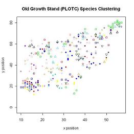
Along with the frequency, the relative location was available for each species in each plot, therefore a clustering coefficient for each species in each plot could be generated. The data collected was based on the presence of a species within each of the 5mx5m subplots in each of the 3 stands. The original 5mx5m subplots were not large enough to capture species clustering, even though visually species clustering could be observed, so the subplots had to be enlarged. FIGURE 6 shows the clustering in the Old Growth Stand. The maximum size of a subplot was set at 40mx40m since anything larger incorrectly determined clustering was occurring. Since the data was collected in 5mx5m subplots and clustering analysis on subplots of this size did not realistically capture the clustering occurring in each stand, subplots sized between 10mx10m and 40mx40m were analyzed. The optimal subplot size needed to captured reasonable clustering within each stand without including large areas outside the sampled stand which data was not avaliable for.
Once the optimal subplot size was established then each of the stands was divided into subplots that best fit the shape of the stand. The Young Growth stand (PLOTA) and the Mid Growth stand (PLOTB) were both divided into 24 subplots and the Old Growth stand (PLOTC) was divided into 70 subplots.
FIGURE 6
Morisita's Index was used to calculate a clustering value for each species in each stand. Morisita's Index was used because it gave a clear value of clustering for each species and did not include the effect of neighbouring subplots in its calculation. Since the exact location of each specimen was not recorded during the data collection but rather the presence of the species within the 5mx5m subplot, increasing the the size of the subplots drastically skewed any neighbouring effect from adjacent subplots. If the neighbouring effect was considered presence of one individual on another could result as high although the actual distance between the individuals is large.
The Morisita's Index is used to get a value for the level of clustering within a area. The formula is as follows:
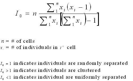
An R Program was written to calculate the Morisita's Index for each species in each stand. Once the frequency of each species in each subplot was determined the vector of values was run through the Morisita function and a clustering value was outputted. This process was repeated for each species in each stand where the frequency of the species in stand.
The distribution of the dbh's of a species within each stand were analyzed to indicate the successional classification of each species. The dbh data for each species was represented as a ratio of the distribution of the dbh in each stand. The dbh of each specimen were categorized into 5cm ranks and then the distribution of individuals within each rank was graphed. This process was repeated for each species in each stand where the frequency of the species in the stand was greater then or equal to 5 individuals. The slope of the graph from the highest point to the lowest point was calculated based on the shape of the distribution. The slopes were then used as the dbh variable for each species in each stand.
The following criteria was used to distinguish the shape of each successional classification in each stand to calculate
the slope of the dbh distribution of each species:
PLOTA
-Young Growth Stand
EARLY SUCCESSIONAL - High frequency of small specimens with a negative distribution slope
PLOTB
-Mid Growth Stand
EARLY SUCCESSIONAL - Low frequency of small specimens with a positive distribution slope
PLOTC
-Late Growth Stand
EARLY SUCCESSIONAL - Very Low frequency of small specimens with a positive distribution slope Select the stand title for graphic examples of species
within the stand
Since all of the species did not have 5 or more individuals present calculating the clustering and dbh
variables produced an incomplete data set. An incomplete data set
cannot be used in multivariate analyses so the significance of each variable in classifying early, mid and late
successional species was tested by comparing correlations and mean values for each variable for species whose
succession classification was known.
Early successional species were
hypothesized to have high frequency and negative dbh slopes in the Young Growth stand (PLOTA) and high clustering and positive
dhb slopes in the Old Growth stand (PLOTC). Mid successional species were hypothesized to have high frequency and negative dbh
slopes in the Mid Growth stand (PLOTB) and 0 dbh slope in the Old Growth stand (PLOTC). Late successional species were hypothesized
to have high frequency and negative dbh slope in the Old Growth stand (PLOTC), low frequency and high clustering in the Young
Growth stand (PLOTA), and negative slopes in all three stands. The hypothesis for each succession classification was derived from basic traits of early, mid a
late successional species.
HOME
MID SUCCESSIONAL - Low frequency of small specimens with a negative distribution slope
LATE SUCCESSIONAL - Very low frequency of small specimens with a negative distribution slope
MID SUCCESSIONAL - High frequency of small specimens with a negative distribution slope
LATE SUCCESSIONAL - Low frequency of small specimens with a negative distribution slope
MID SUCCESSIONAL - Low frequency of small specimens with a zero distribution slope
LATE SUCCESSIONAL - High frequency of small specimens with a negative distribution slope
Data Preparation Methods: Determining Significant
Variables for Multivariate Analyses
INTRODUCTION
DATA DETAILS
MULTIVARIATE METHODS
MULTIVARIATE RESULTS & DISCUSSION
CONCLUSION
APPENDICES
REFERENCES & ACKNOWLEDGEMENTS
DATA PREPARATION METHODS
DATA PREPARATION RESULTS & DISCUSSION
PRELIMINARY ANALYSIS