function (a,b,c) {

dij=1-(a/(a+b+c))

print("Dissimilarity Coefficient: ")
print(dij)
}
To run the program I manually counted the number of species that were common and the number of species that were different amongst
the subplots of interest and entered those values into the program. The outputs from this analysis showed that my hypothesis that
clustering was occurring in the south-west corner of the Old Growth stand (PLOTC) was true and I was able to draw a border around the
cluster.
FIGURE 14
shows the Old Growth stand Plot including the cluster border. From this image and the work I had previously done, I was able to
identify 12 species that fell within the border.
 FIGURE 14
The second stage of this analysis was to determine the spatial autocorrelation between the 12 species of interest. To calculate the
autocorrelation I used the Moran's I Autocorrelation Statistic, but I had to reformat the equation since it is generally used to measure
the spatial autocorrelation between subplots not species. I reformatted the Moran's I statistic to be the following:
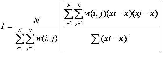
where xi = number of sub-plots species i is located in, xj = number of sub-plots species j is located in, = average number of plots
that have both species present, = the ij-value of the NxN spatial weight matrix and N = total number of sub-plots.
The weight matrix, W, is matrix that show the relationship between sub-plots that are neighbours. Each entry in the matrix is the number
of neighbouring sub-plots that contain the species. Outputs from the equation will lie between -1 (negatively correlated) and 1 (positively
correlated).
Writing a program in R to calculate the Moran's I statistic was quite complicated because I had to account for neighbouring within a cell if
the species I was analyzing were both present in the same cell. It was easier to calculate the Moran's I statistic by hand. This was
extremely time consuming, because the neighbouring values had to be counted for each occurrence of a species in relationship to the second species
being analyzed. Since there were 12 species of interest this process had to be repeated a large number of times for both the Young Growth stand
(PLOTA) and the Mid Growth stand (PLOTB). From my analysis I calculated the spatial autocorrelation between the species Bagokon and
Balante and the spatial autocorrelation between Bagokon and Biri to be 4.45112 and 3.221 which are incorrect. As a result of calculating these
values I reevaluated my analysis and determined that my logic and my reformation of the Moran I statistic was flawed.
I wanted to conduct an analysis that still focused around determining a species’ successional classification because I felt that by determining
the classification it could lead to the primary goal of relieving stress on Old Growth forests in the Philippines by illegal loggers. While my initial
ideas on how to conduct this analysis did not work some of the work that I put into the analysis help in the final analysis of this project. The hand work
I did to determine the size of subplots within the Old Growth stand (PLOTC) and record the presence of species within the subplots helped to
determine the optimal size of subplots for the Morisita's Index cluster analysis. Although the initial plan for this project did not work it evolved
it to an analysis that better fit the data and provided more ecologically relevant information.
HOME
INTRODUCTION
DATA DETAILS
MULTIVARIATE METHODS
MULTIVARIATE RESULTS & DISCUSSION
CONCLUSION
APPENDICES
REFERENCES & ACKNOWLEDGEMENTS
DATA PREPARATION METHODS
DATA PREPARATION RESULTS & DISCUSSION
PRELIMINARY ANALYSIS